Create a time series anomaly prediction experiment to train a model that can detect anomalies, or unexpected results, when the model predicts results based on new data.
Tech preview This is a technology preview and is not yet supported for use in production environments.
Detecting anomalies in predictions
You can use anomaly prediction to find outliers in model predictions. Consider the following scenarios for training a time series model with anomaly prediction. For example, suppose you have operational metrics from monitoring devices that were collected in the date range of 2022.1.1 through 2022.3.31. You are confident that no anomalies exist in the data for that period, even if the data is unlabeled. You can use a time series anomaly prediction experiment to:
- Train model candidate pipelines and auto-select the top-ranked model candidate
- Deploy a selected model to predict new observations if:
- A new time point is an anomaly (for example, an online score predicts a time point 2022.4.1 that is outside of the expected range)
- A new time range has anomalies (for example, a batch score predicts values of 2022.4.1 to 2022.4.7, outside the expected range)
Working with a sample
To create an AutoAI Time series experiment with anomaly prediction that uses a sample:
-
Create an AutoAI experiment.
-
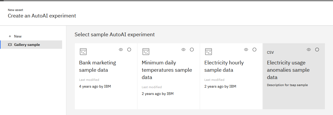
Select Resource hub sample.

-
Click the tile for Electricity usage anomalies sample data.
-
Follow the prompts to configure and run the experiment.

-
Review the details about the pipelines and explore the visualizations.
Configuring a time series experiment with anomaly prediction
-
Load the data for your experiment.
Restriction: You can upload only a single data file for an anomaly prediction experiment. If you upload a second data file (for holdout data) the Anomaly prediction option is disabled, and only the Forecast option is available. By default, Anomaly prediction experiments use a subset of the training data for validation. -
Click Yes to Enable time series.
-
Select Anomaly prediction as the experiment type.
-
Configure the feature columns from the data source that you want to predict based on the previous values. You can specify one or more columns to predict.
-
Select the date/time column.
The prediction summary shows you the experiment type and the metric that is selected for optimizing the experiment.
Configuring experiment settings
To configure more details for your time series experiment, open the Experiment settings pane. Options that are not available for anomaly prediction experiments are unavailable.
General prediction settings
On the General panel for prediction settings, configure details for training the experiment.
| Field | Description |
|---|---|
| Prediction type | View or change the prediction type based on prediction column for your experiment. For time series experiments, Time series anomaly prediction is selected by default. Note: If you change the prediction type, other prediction settings for your experiment are automatically changed. |
| Optimized metric | Choose a metric for optimizing and ranking the pipelines. |
| Optimized algorithm selection | Not supported for time series experiments. |
| Algorithms to include | Select algorithms based on which you want your experiment to create pipelines. The algorithms support anomaly prediction. |
| Pipelines to complete | View or change the number of pipelines to generate for your experiment. |
Time series configuration details
On the Time series pane for prediction settings, configure the details for how to train the experiment and generate predictions.
| Field | Description |
|---|---|
| Date/time column | View or change the date/time column for the experiment. |
| Lookback window | Not supported for anomaly prediction. |
| Forecast window | Not supported for anomaly prediction. |
Configuring data source settings
To configure details for your input data, open the Experiment settings panel and select the Data source.
General data source settings
On the General panel for data source settings, you can choose options for how to use your experiment data.
| Field | Description |
|---|---|
| Duplicate rows | Not supported for time series anomaly prediction experiments. |
| Subsample data | Not supported for time series anomaly prediction experiments. |
| Text feature engineering | Not supported for time series anomaly prediction experiments. |
| Final training data set | Anomaly prediction uses a single data source file, which is the final training data set. |
| Supporting features | Not supported for time series anomaly prediction experiments. |
| Data imputation | Not supported for time series anomaly prediction experiments. |
| Training and holdout data | Anomaly prediction does not support a separate holdout file. You can adjust how the data is split between training and holdout data. Note: In some cases, AutoAI can overwrite your holdout settings to ensure the split is valid for the experiment. In this case, you see a notification and the change is noted in the log file. |
Reviewing the experiment results
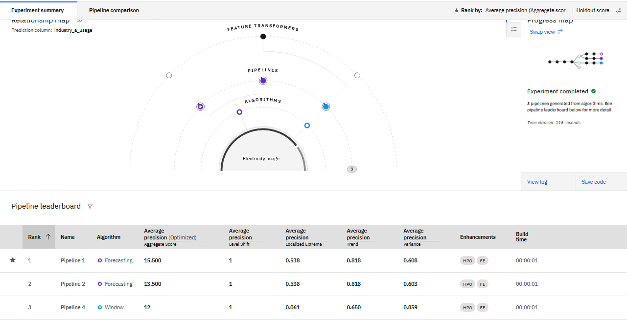
When you run the experiment, the progress indicator displays the pathways to pipeline creation. Ranked pipelines are listed on the leaderboard. Pipeline score represents how well the pipeline performed for the optimizing metric.
The Experiment summary tab displays a visualization of how metrics performed for the pipeline.
- Use the metric filter to focus on particular metrics.
- Hover over the name of a metric to view details.
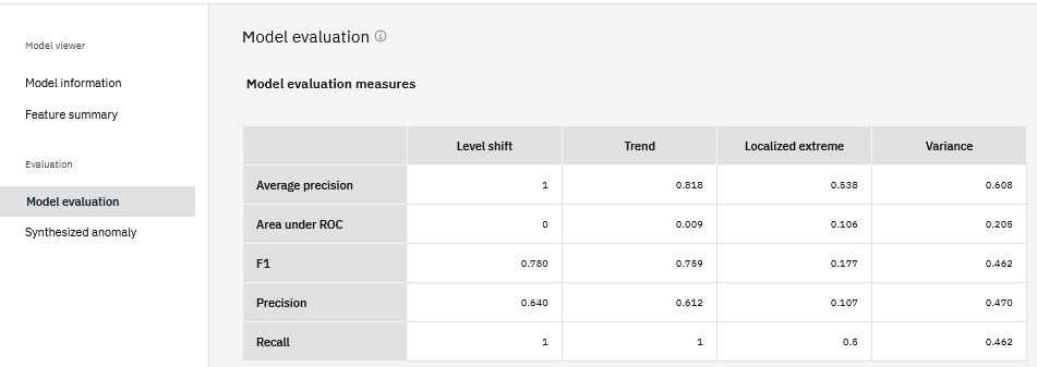
Click a pipeline name to view details. On the Model evaluation page, you can review a table that summarizes details about the pipeline.

- The rows represent five evaluation metrics: Area under ROC, Precision, Recall, F1, Average precision.
- The columns represent four synthesized anomaly types: Level shift, Trend, Localized extreme, Variance.
- Each value in a cell is an average of the metric based on three iterations of evaluation on the synthesized anomaly type.
Evaluation metrics:
These metrics are used to evaluate a pipeline:
| Metric | Description |
|---|---|
| Aggregate score (Recommended) | This score is calculated based on an aggregation of the optimized metric (for example, Average precision) values for the 4 anomaly types. The scores for each pipeline are ranked, using the Borda count method, and then weighted for their contribution to the aggregate score. Unlike a standard metric score, this value is not between 0 and 1. A higher value indicates a stronger score. |
| ROC AUC | Measure of how well a parameter can distinguish between two groups. |
| F1 | Harmonic average of the precision and recall, with best value of 1 (perfect precision and recall) and worst at 0. |
| Precision | Measures the accuracy of a prediction based on percent of positive predictions that are correct. |
| Recall | Measures the percentage of identified positive predictions against possible positives in data set. |
Anomaly types
These are the anomaly types AutoAI detects.
| Anomaly type | Description |
|---|---|
| Localized extreme anomaly | An unusual data point in a time series, which deviates significantly from the data points around it. |
| Level shift anomaly | A segment in which the mean value of a time series is changed. |
| Trend anomaly | A segment of time series, which has a trend change compared to the time series before the segment. |
| Variance anomaly | A segment of time series in which the variance of a time series is changed. |
Saving a pipeline as a model
To save a model candidate pipeline as a machine learning model, select Save as model for the pipeline you prefer. The model is saved as a project asset. You can promote the model to a space and create a deployment for it.
Saving a pipeline as a notebook
To review the code for a pipeline, select Save as notebook for a pipeline. An automatically generated notebook is saved as a project asset. Review the code to explore how the pipeline was generated.
For details on the methods used in the pipeline code, see the documentation for the autoai-ts-libs library.
Scoring the model
After you save a pipeline as a model, then promote the model to a space, you can score the model to generate predictions for input, or payload, data. Scoring the model and interpreting the results is similar to scoring a binary classification model, as the score presents one of two possible values for each prediction:
- 1 = no anomaly detected
- -1 = anomaly detected
Deployment details
Note these requirements for deploying an anomaly prediction model.
- The schema for the deplyment input data must match the schema for the training data except for the prediction, or target column.
- The order of the fields for model scoring must be the same as the order of the fields in the training data schema.
Deployment example
The following is valid input for an anomaly prediction model:
{
    "input_data": [
        {
            "id": "observations",
            "values": [
                [12,34],
                [22,23],
                [35,45],
                [46,34]
            ]
        }
     ]
}
The score for this input is [1,1,-1,1] where -1 means the value is an anomaly and 1 means the prediction is in the normal range.
Implementation details
These algorithms support anomaly prediction in time series experiments.
| Algorithm | Type | Transformer |
|---|---|---|
| Pipeline Name | Algorithm Type | Transformer |
| PointwiseBoundedHoltWintersAdditive | Forecasting | N/A |
| PointwiseBoundedBATS | Forecasting | N/A |
| PointwiseBoundedBATSForceUpdate | Forecasting | N/A |
| WindowNN | Window | Flatten |
| WindowPCA | Relationship | Flatten |
| WindowLOF | Window | Flatten |
The algorithms are organized in these categories:
- Forecasting: Algorithms for detecting anomalies using time series forecasting methods
- Relationship: Algorithms for detecting anomalies by analyzing the relationship among data points
- Window: Algorithms for detecting anomalies by applying transformations and ML techniques to rolling windows
Learn more
Saving an AutoAI generated notebook (Watson Machine Learning)
Parent topic: Building a time series experiment