You can create, train, and deploy models using SPSS Modeler. Read about SPSS Modeler, then watch a video and follow a tutorial that’s suitable for beginners and requires no coding.
- Required services
- watsonx.ai Studio (which includes SPSS Modeler)
- watsonx.ai Runtime
Your basic workflow includes these tasks:
- Create a project. Projects are where you can collaborate with others to work with data.
- Add an SPSS Modeler flow to the project.
- Configure the nodes on the canvas, and run the flow.
- Review the model details and save the model.
- Deploy and test your model.
Read about SPSS Modeler
With SPSS Modeler flows, you can quickly develop predictive models using business expertise and deploy them into business operations to improve decision making. Designed around the long-established SPSS Modeler client software and the industry-standard CRISP-DM model it uses, the flows interface facilitates the entire data mining process, from data to better business results.
SPSS Modeler offers a variety of modeling methods taken from machine learning, artificial intelligence, and statistics. The methods available on the node palette allow you to derive new information from your data and to develop predictive models. Each method has certain strengths and is best suited for particular types of problems.
Watch a video about creating a model using SPSS Modeler
 Watch this video to see how to create and run an SPSS Modeler flow to train a machine learning model.
This video provides a visual method to learn the concepts and tasks in this documentation.
Try a tutorial to create a model using SPSS Modeler
In this tutorial, you will complete these tasks:
- Task 1: Open a project.
- Task 2: Add a data set to your project.
- Task 3: Create the SPSS Modeler flow.
- Task 4: Add the nodes to the SPSS Modeler flow.
- Task 5: Run the SPSS Modeler flow and explore the model details.
- Task 6: Evaluate the model.
- Task 7: Deploy and test the model with new data.
This tutorial will take approximately 30 minutes to complete.
Example data
The data set used in this tutorial is from the University of California, Irvine, and is the result of an extensive study based on hospital admissions over a period of time. The model will use three important factors to help predict chronic kidney disease.
Tips for completing this tutorial
Here are some tips for successfully completing this tutorial.
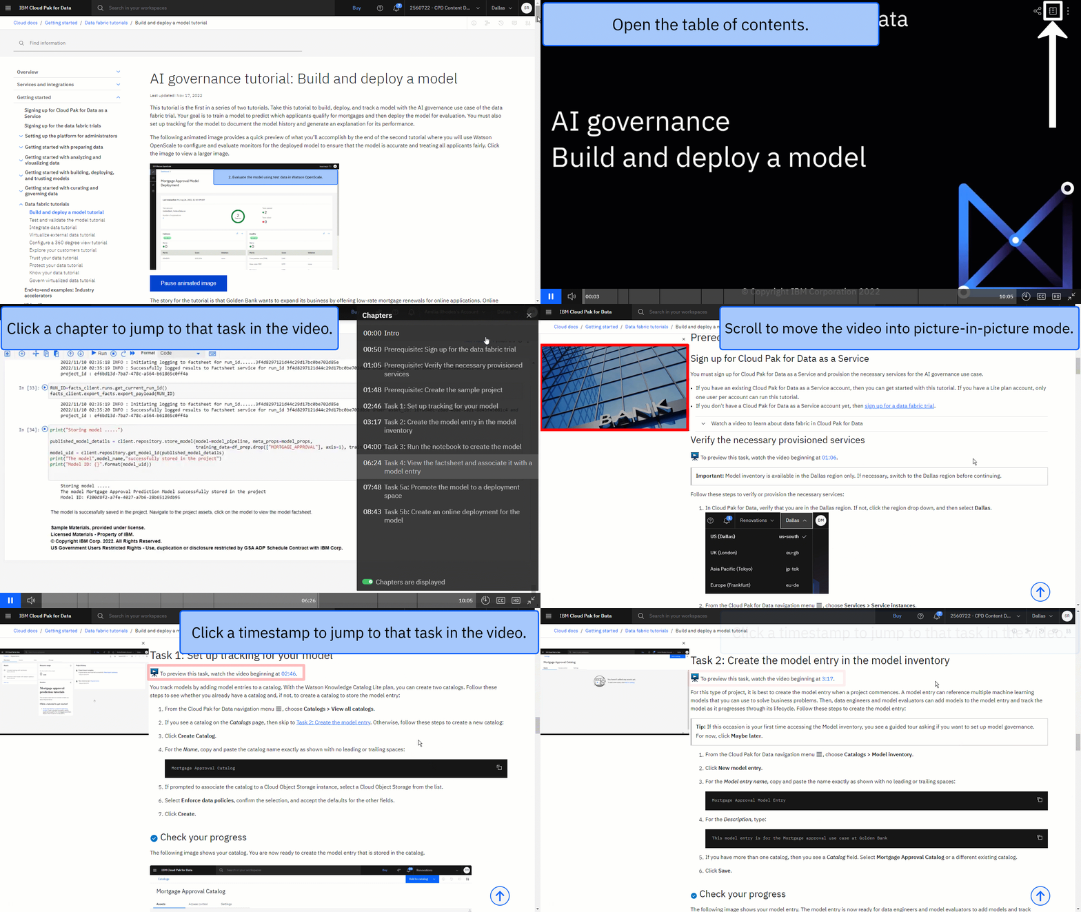
Use the video picture-in-picture
The following animated image shows how to use the video picture-in-picture and table of contents features:
Get help in the community
If you need help with this tutorial, you can ask a question or find an answer in the Cloud Pak for Data Community discussion forum.
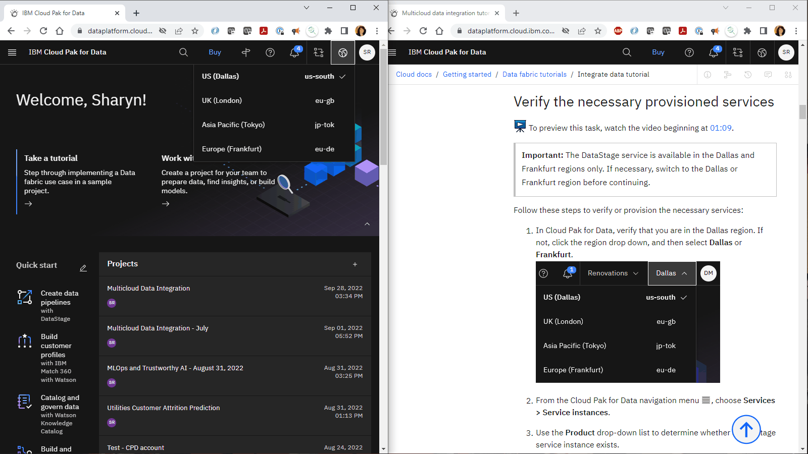
Set up your browser windows
For the optimal experience completing this tutorial, open Cloud Pak for Data in one browser window, and keep this tutorial page open in another browser window to switch easily between the two applications. Consider arranging the two browser windows side-by-side to make it easier to follow along.
Task 1: Open a project
You need a project to store the SPSS Modeler flow. You can use an existing project or create a project.
-
From the Navigation Menu
, choose Projects > View all projects
-
Open an existing project. If you want to use a new project:
-
Click New project.
-
Select Create an empty project.
-
Enter a name and optional description for the project.
-
Choose an existing object storage service instance or create a new one.
-
Click Create.
-
For more information or to watch a video, see Creating a project.
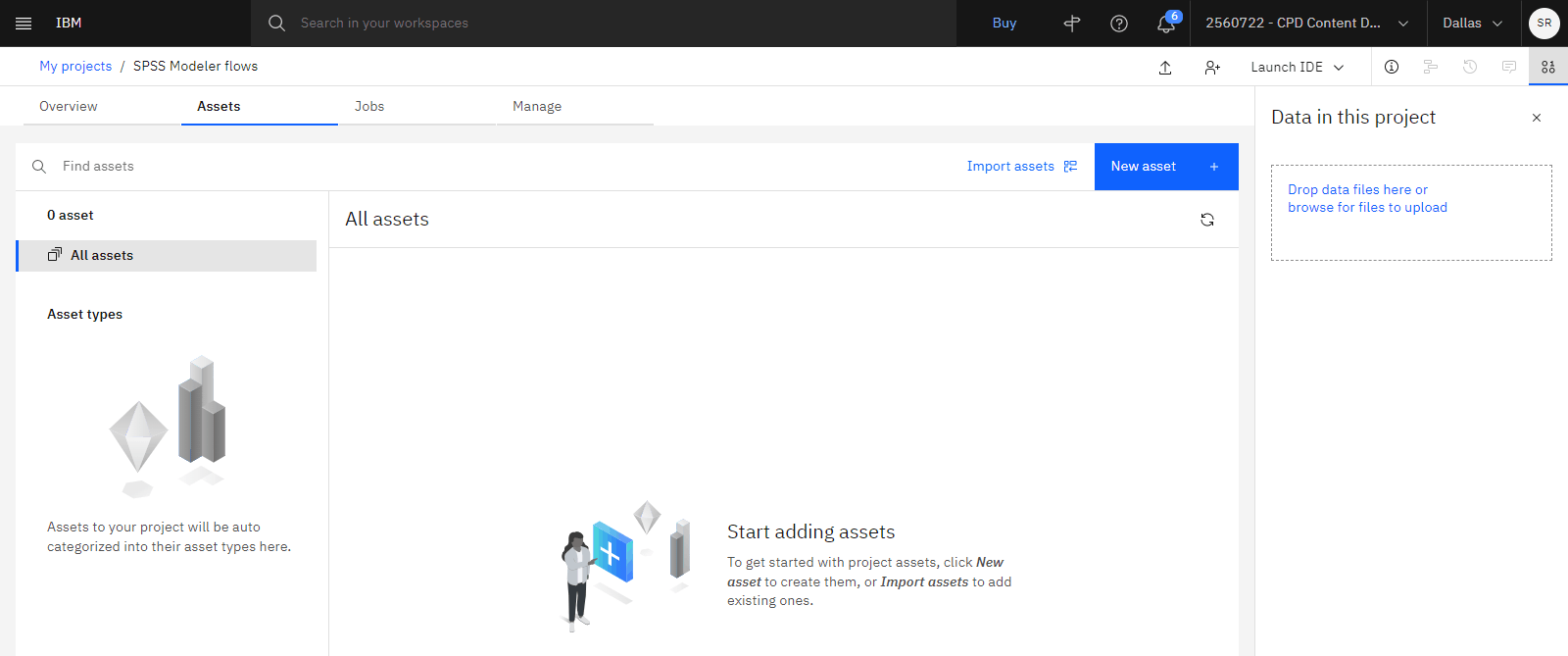
 Check your progress
The following image shows the new project.
Task 2: Add the data set to your project
 To preview this task, watch the video beginning at 00:13.
This tutorial uses a sample data set. Follow these steps to add the sample data set to your project:
-
Access the UCI ML Repository: Chronic Kidney Disease Data Set in the Resource hub.
-
Click Preview. There are three important factors that help predict chronic kidney disease which are available as part of this analysis: the age of the test subject, the serum creatinine test results, and diabetes test results. And the class value indicates if the patient has been previously diagnosed for kidney disease.
-
Click Add to project.
-
Select the project from the list, and click Add.
-
Click View Project.
-
From your project's Assets page, locate the UCI ML Repository Chronic Kidney Disease Data Set.csv file.
 Check your progress
The following image shows the Assets tab in the project.

Task 3: Create the SPSS Modeler flow
 To preview this task, watch the video beginning at 01:11.
Follow these steps to create an SPSS Modeler flow in the project:
-
Click New asset > Build models as a visual flow.
-
Type a name and description for the flow.
-
For the runtime definition, accept the Default SPSS Modeler S definition.
-
Click Create. This opens up the Flow Editor that you'll use to create the flow.
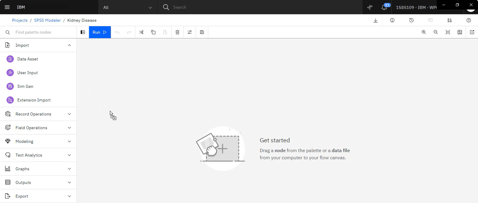
 Check your progress
The following image shows the flow editor.
Task 4: Add the nodes to the SPSS Modeler flow
 To preview this task, watch the video beginning at 01:31.
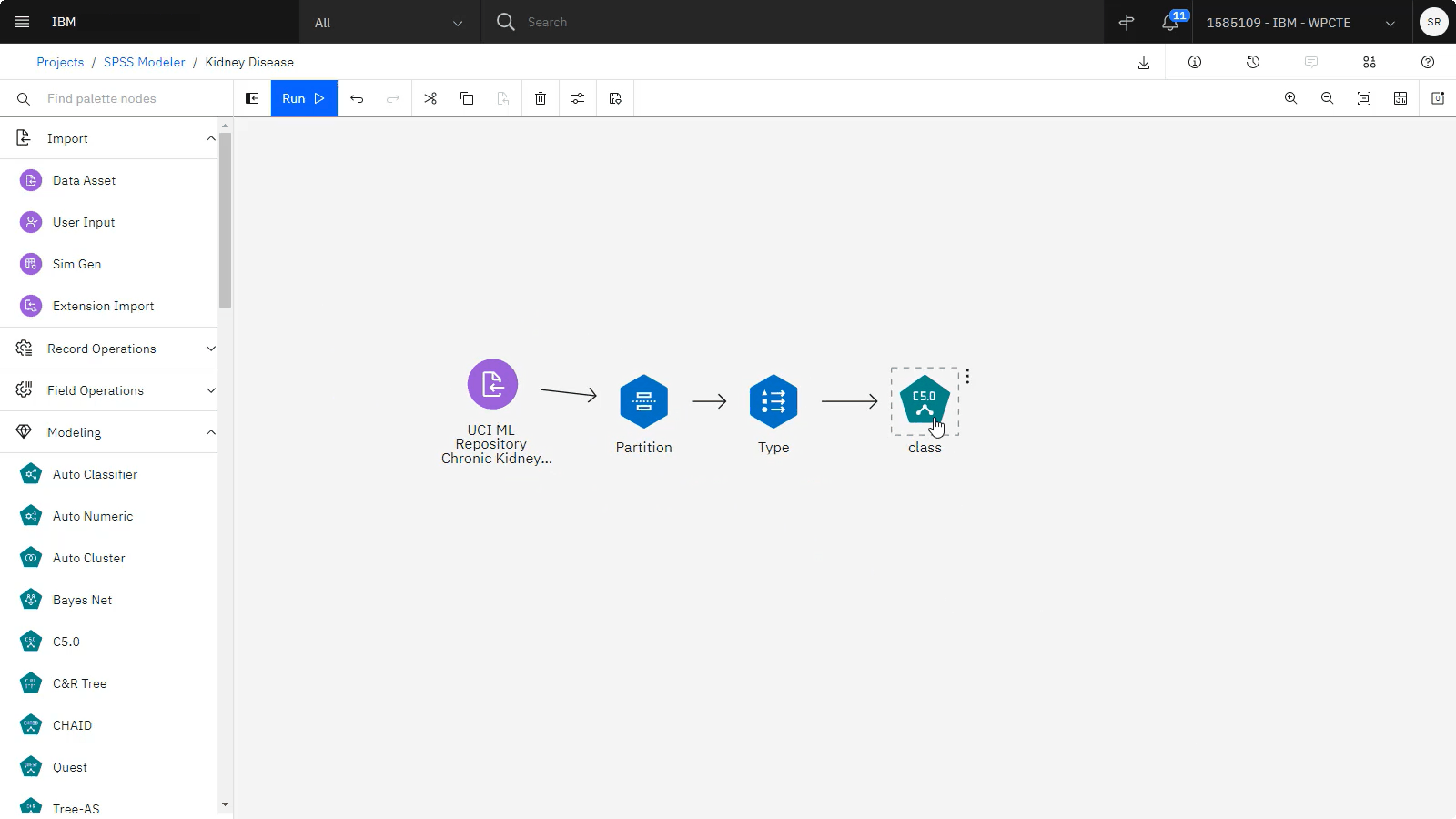
After you load the data, you must transform the data. Create a simple flow by dragging transformers and estimators onto the canvas and connecting them to the data source. Use the following nodes from the palette:
-
Data Asset: loads the csv file from the project
-
Partition: divides the data into training and testing segments
-
Type: sets the data type. Use it to designate the
classfield as atargettype. -
C5.0: a classification algorithm
-
Analysis: view the model and check its accuracy
-
Table: preview the data with predictions
Follow these steps to create the flow:
-
Add the data asset node:
-
From the Import section, drag the Data Asset node onto the canvas.
-
Double-click the Data Asset node to select the data set.
-
Select Data asset > UCI ML Repository Chronic Kidney Disease Data Set.csv.
-
Click Select.
-
View the Data Asset properties.
-
Click Save.
-
-
Add the Partition node:
-
From the Field Operations section, drag the Partition node onto the canvas.
-
Connect the Data Asset node to the Partition node.
-
Double-click the Partition node to view its properties. The default partition divides half of the data for training and the other half for testing.
-
Click Save.
-
-
Add the Type node:
-
From the Field Operations section, drag the Type node onto the canvas.
-
Connect the Partition node to the Type node.
-
Double-click the Type node to view its properties. The Type node specifies the measurement level for each field. This source data file uses four different measurement levels: Continuous, Categorical, Nominal, Ordinal, and Flag.
-
Search for the
classfield. For each field, the role indicates the part that each field plays in modeling. Change theclassRole to Target - the field you want to predict. -
Click Save.
-
-
Add the C5.0 classification algorithm node:
-
From the Modeling section, drag the C5.0 node onto the canvas.
-
Connect the Type node to the C5.0 node.
-
Double-click the C5.0 node to view its properties. By default, the C5.0 algorithm builds a decision tree. A C5.0 model works by splitting the sample based on the field that provides the maximum information gain. Each sub-sample defined by the first split is then split again, usually based on a different field, and the process repeats until the subsamples can't be split any further. Finally, the lowest-level splits are reexamined, and those that don't contribute significantly to the value of the model are removed.
-
Toggle on Use settings defined in this node.
-
For Target, select class.
-
In the Inputs section, click Add columns.
-
Clear the checkbox next to Field name.
-
Select age, sc, dm.
-
Click OK.
-
-
Click Save.
-
 Check your progress
The following image shows the completed flow.
Task 5: Run the SPSS Modeler flow and explore the model details
 To preview this task, watch the video beginning at 04:20.
Now that you have designed the flow, follow these steps to run the flow, and examine the tree diagram to see the decision points:
-
Right-click the C5.0 node and select Run. Running the flow generates a new model nugget on the canvas.
-
Right-click the model nugget and select View Model to view the model details.
-
View the Model Information which provides a model summary.
-
Click Top Decision Rules. A table displays a series of rules that were used to assign individual records to child nodes based on the values of different input fields.
-
Click Feature Importance. A chart shows the relative importance of each predictor in estimating the model. From this, you can see that serum creatinine is easily the most significant factor, with diabetes being the next most significant factor.
-
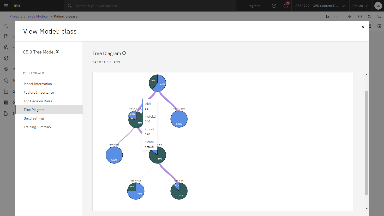
Click Tree Diagram. The same model is displayed in the form of a tree, with a node at each decision point.
-
Hover over the top node, which provides a summary for all the records in the data set. Almost 40% of the cases in the data set are classified as not diagnosed with kidney disease. The tree can provide additional clues as to what factors might be responsible.
-
Notice the two branches stemming from the top node, which indicates a split by serum creatinine.
-
Review the branch that shows records where the serum creatinine is greater than 1.25. In this case, 100% of those patients have a positive kidney disease diagnosis.
-
Review the branch that shows records where the serum creatinine is less than or equal to 1.25. Almost 80% of those patients don't have a positive kidney disease diagnosis, but almost 20% with lower serum creatinine were still diagnosed with kidney disease.
-
-
Notice the branches stemming from sc<=1.250, which is split by diabetes.
-
Review the branch that shows patients with low serum creatinine (sc<=1.250) and diagnosed diabetes (dm=yes). 100% of these patients were also diagnosed with kidney disease.
-
Review the branch that shows patients with low serum creatinine (sc<=1.250) and no diabetes (dm=no), 85% were not diagnosed with kidney disease, but 15% of them were still diagnosed with kidney disease.
-
-
Notice the branches stemming from dm = no, which is split by the last significant factor, age.
-
Review the branch that shows patients 14 years old or younger (age <= 14). This branch shows that 75% of young patients with low serum creatinine and no diabetes were at risk of getting kidney disease.
-
Review the branch that shows patients older than 14 years old (age > 14). This branch shows that only 12% of patients over 14 years old with low serum creatinine and no diabetes were at risk of getting kidney disease.
-
-
Close the model details.
-
 Check your progress
The following image shows the tree diagram.
Task 6: Evaluate the model
 To preview this task, watch the video beginning at 07:24.
Follow these steps to use the Analysis and Table nodes to evaluate the model:
-
From the Outputs section, drag the Analysis node onto the canvas.
-
Connect the Model nugget to the Analysis node.
-
Right-click the Analysis node, and select Run.
-
From the Outputs panel, open the Analysis, which shows that the model correctly predicted a kidney disease diagnosis almost 95% of the time. Close the Analysis.
-
(Optional) On the toolbar, click the Download icon to save the model as an .str file.
-
Right-click the Analysis node, and select Save branch as a model.
-
For the Model name, type
Kidney Disease Analysis. -
Click Save.
-
Click Close.
-
-
From the Outputs section, drag the Table node onto the canvas.
-
Connect the Model nugget to the Table node.
-
Right-click the Table node, and select Preview data.
-
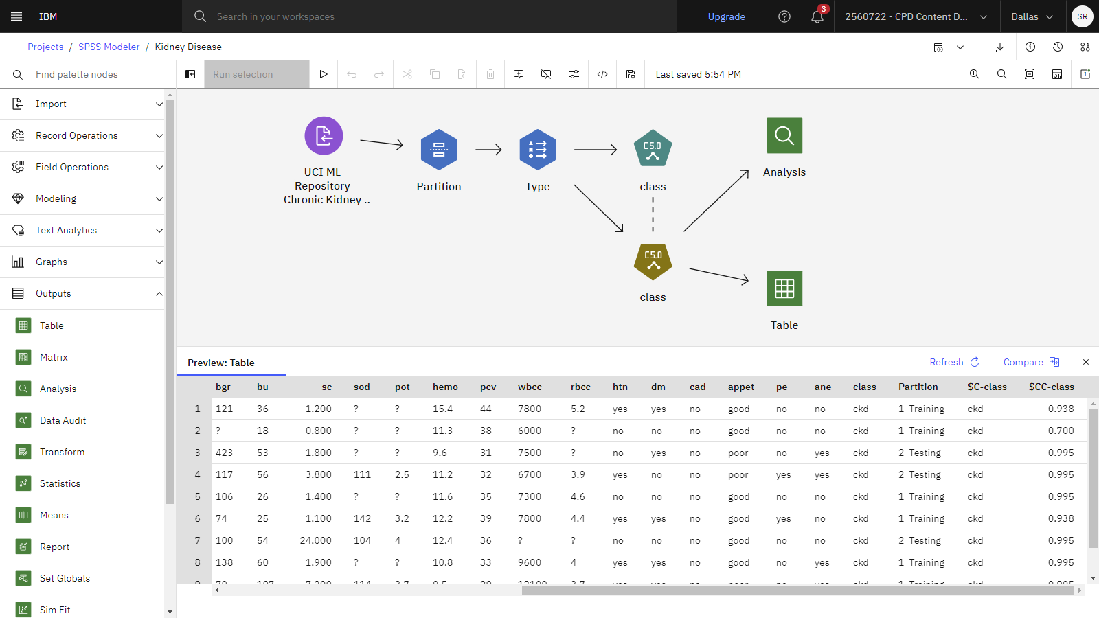
When the Preview displays, scroll to the last two columns. The $C-Class column contains the prediction of kidney disease, and the $CC-Class column indicates the confidence score for that prediction.
-
Close the Preview.
-
 Check your progress
The following image shows the preview table with the predictions.
Task 7: Deploy and test the model with new data
 To preview this task, watch the video beginning at 09:10.
Lastly, follow these steps to deploy this model and predict the outcome with new data.
-
Return to the Project's Assets tab.
-
Click the Models section, and open the Kidney Disease Analysis model.
-
Click the Promote to deployment space icon
.
-
Choose an existing deployment space. If you don't have a deployment space, you can create a new one:
-
Provide a space name.
-
Select a storage service.
-
Select a machine learning service.
-
Click Create.
-
Click Close.
-
-
Select Go to the model in the space after promoting it.
-
Click Promote.
-
When the model displays inside the deployment space, click New deployment.
-
Select Online as the Deployment type.
-
Specify a name for the deployment.
-
Click Create.
-
-
When the deployment is complete, click the deployment name to view the deployment details page.
-
Go to the Test tab. You can test the deployed model from the deployment details page in two ways: test with a form or test with JSON code.
-
Click the JSON input, then copy the following test data and paste it to replace the existing JSON text:
{ "input_data": [ { "fields": [ "age", "bp", "sg", "al", "su", "rbc", "pc", "pcc", "ba", "bgr", "bu", "sc", "sod", "pot", "hemo", "pcv", "wbcc", "rbcc", "htn", "dm", "cad", "appet", "pe", "ane", "class" ], "values": [ [ "62", "80", "1.01", "2", "3", "normal", "normal", "notpresent", "notpresent", "423", "53", "1.8", "", "", "9.6", "31", "7500", "", "no", "yes", "no", "poor", "no", "yes", "ckd" ] ] } ] } -
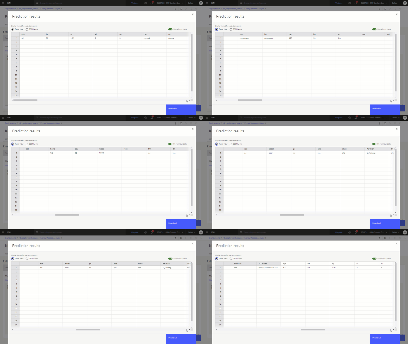
Click Predict to predict whether a 62 year old with diabetes and a serum creatinine ratio of 1.8 would likely be diagnosed with kidney disease. The resulting prediction indicates that this patient has a high probability of a kidney disease diagnosis.
 Check your progress
The following image shows the Test tab for the model deployment with a prediction.
Next steps
Now you can use this data set for further analysis. For example, you can perform tasks such as:
Additional resources
-
Find more SPSS Modeler tutorials
-
Try these other methods to build models:
-
View more videos
-
Find sample data sets and notebooks to gain hands-on experience building models in the Resource hub
-
Contribute to the SPSS Modeler community
Parent topic: Quick start tutorials