This tutorial uses the Self-Learning Response Model (SLRM) node, which generates and enables the updating of a model to predict which offers are most appropriate for customers and the probability of the offers being accepted. These sorts of models are most beneficial in customer relationship management, such as marketing applications or call centers.
This example is based on a fictional banking company. The marketing department wants to achieve more profitable results in future campaigns by matching the appropriate offer of financial services to each customer. Specifically, the example uses a Self-Learning Response model to identify the characteristics of customers who are most likely to respond favorably based on previous offers and responses and to promote the best current offer based on the results.
Try the tutorial
In this tutorial, you will complete these tasks:
Sample modeler flow and data set
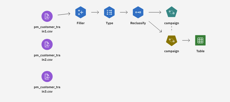
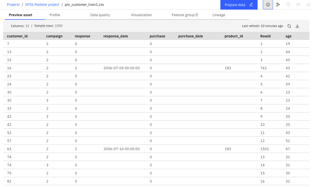
This tutorial uses the Making Offers to Customers - Self-Learning flow in the sample project. The data files that are used are pm_customer_train1.csv, pm_customer_train2.csv, and pm_customer_train3.csv. The following image shows the sample modeler flow.
Task 1: Open the sample project
The sample project contains several data sets and sample modeler flows. If you don't already have the sample project, then refer to the Tutorials topic to create the sample project. Then follow these steps to open the sample project:
- In Cloud Pak for Data, from the Navigation menu
, choose Projects > View all Projects.
- Click SPSS Modeler Project.
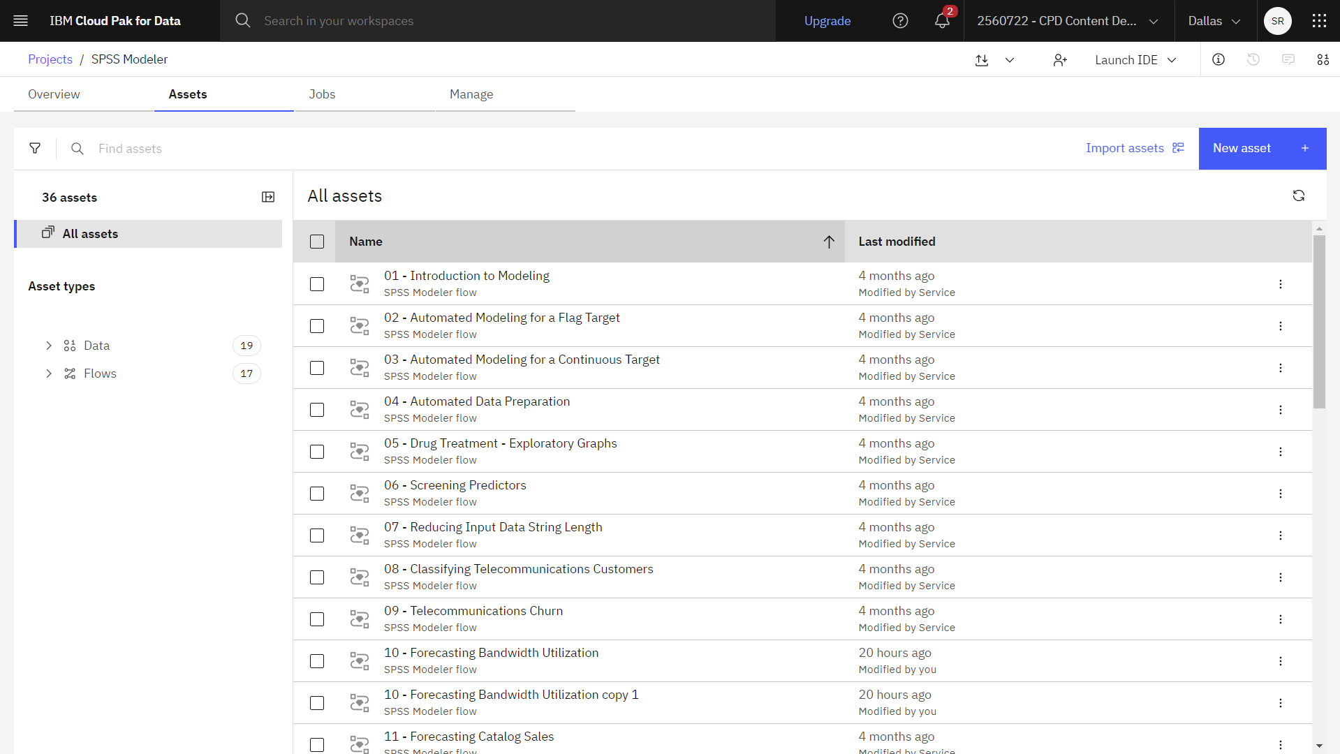
- Click the Assets tab to see the data sets and modeler flows.
Check your progress
The following image shows the project Assets tab. You are now ready to work with the sample modeler flow associated with this tutorial.
Task 2: Examine the Data Asset and Filler node
Making Offers to Customers - Self-Learning modeler flow includes several nodes. Follow these steps to examine the Data Asset and Filler nodes:
- From the Assets tab, open the Making Offers to Customers - Self-Learning modeler flow, and wait for the canvas to load.
- Double-click the pm_customer_train1.csv node. This node is a Data Asset node that points to the pm_customer_train1.csv file in the project.
- Review the File format properties.
- Optional: Click Preview data to see the full data set.
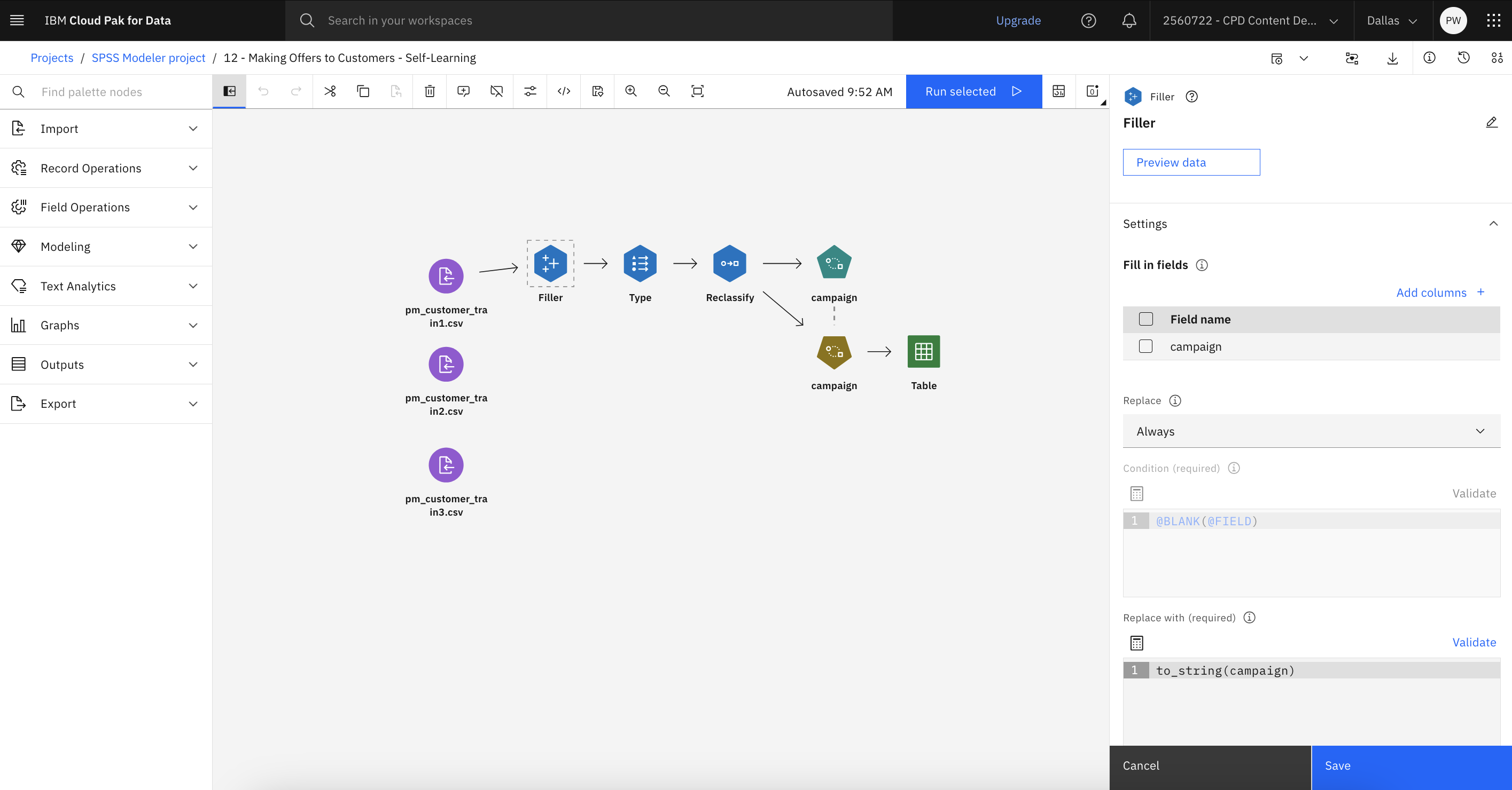
- Double-click the Filler node.
Filler nodes are used to replace field values
and change storage. You can choose to replace values based on a specified CLEM condition, such as
@BLANK(FIELD). Alternatively, you can choose to replace all blanks or null values with a specific value. Filler nodes are often used with the Type node to replace missing values. In the Fill in fields section, you can specify the fields from the dataset whose values you want to be examined and replaced. In this case, thecampaigncolumn is specified together with an Always selection under the Replace section. - Click Cancel.
Check your progress
The following image shows the Filler node. You are now ready to examine the Type and Reclassify nodes.
Task 3: Examine the Type and Reclassify nodes
Follow these steps to examine the Type and Reclassify nodes:
- Double-click the Type node to see its properties.
With the Type node, you can
indicate the types of fields you're using and how they're used to predict the outcomes. Notice, that
the role for the
campaignandresponsefields are set to Target. The specified targets are the fields on which you want to base your predictions. The Measure is set to Flag for theresponsefield. - Click Read values.
Figure 3. Measurement levels 
- Click Save.
Because the campaign field data shows as a list of numbers (1, 2, 3, and 4), you can reclassify the fields to have more meaningful titles.
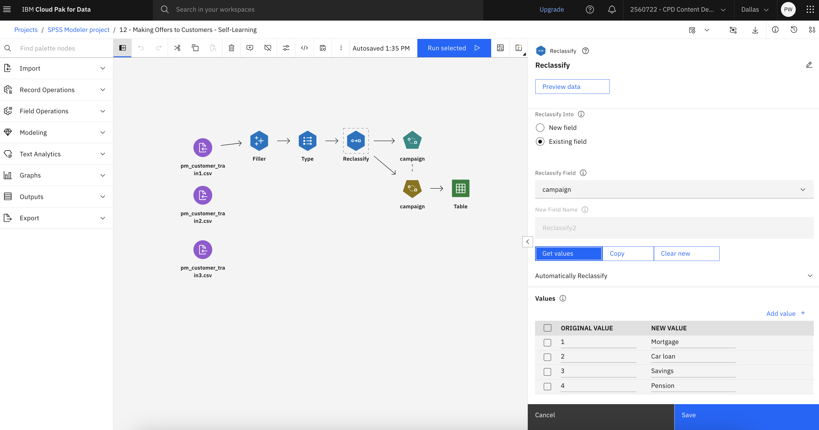
- Double-click the Reclassify node to see its properties.
- In the Reclassify Into section, select Existing field.
- Next, in the Reclassify Field section, select campaign.
- Click Get values. The campaign values are added to the
ORIGINAL
VALUE
column. - Notice, that in the Values section in the
NEW VALUEcolumn, there are four rows:- Mortgage
- Car loan
- Savings
- Pension
- Click Save.
Check your progress
The following image shows the Reclassify node. You are now ready to explore the SLRM node.
Task 4: Explore the SLRM node
Follow these steps to explore the SLRM node:
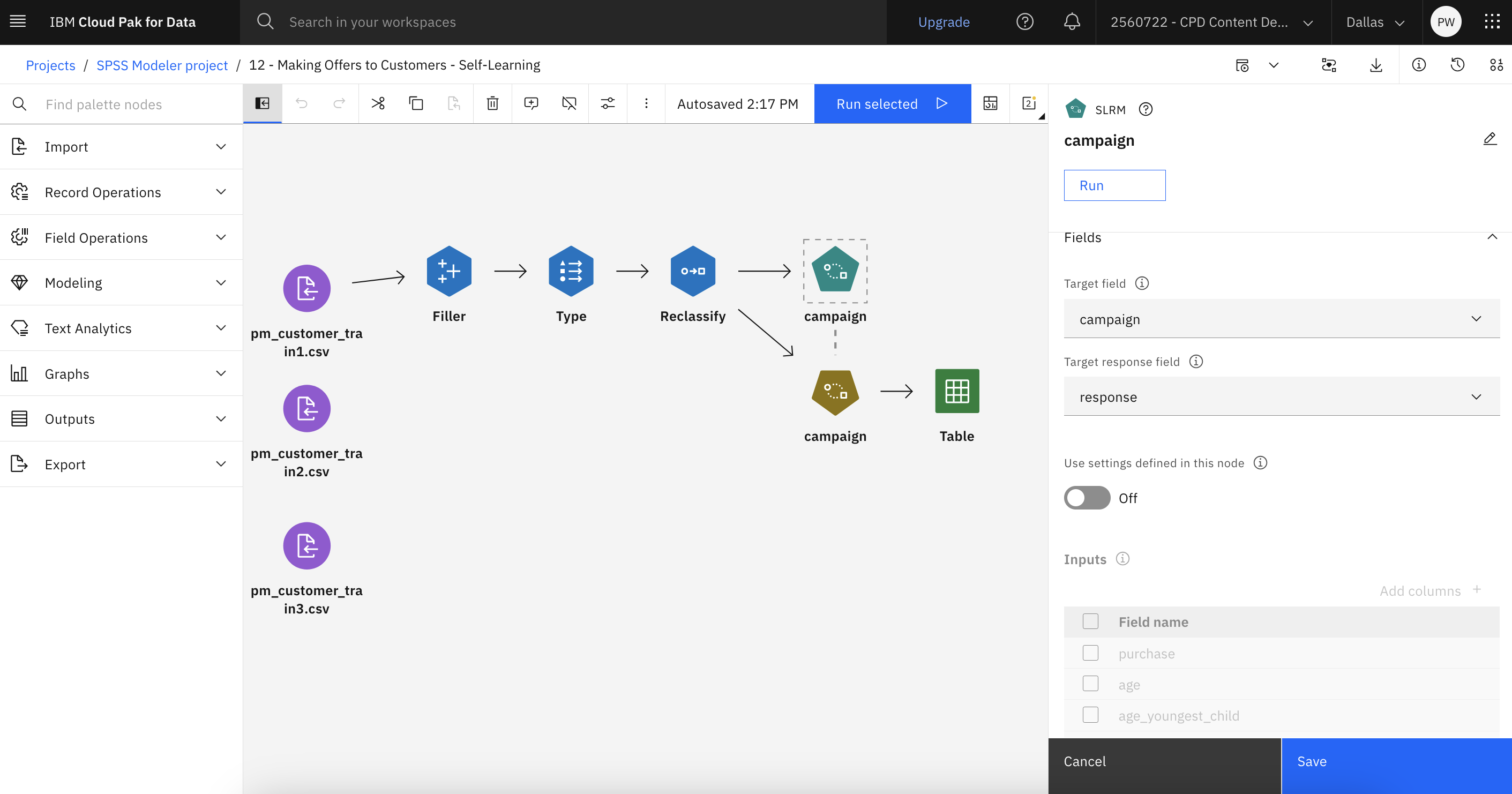
- Double-click the campaign (SLRM) node to view its properties.
- Select
campaignfor the Target field, andresponsefor the Target response field. - Under Model Options, for Maximum number of predictions per record, reduce the number to 2. This means that for each customer there are two offers identified that have the highest probability of being accepted.
- Make sure Take account of model reliability is selected.
- Click Save.
Check your progress
The following image shows the flow. You are now ready to generate the model.
Task 5: Generate the model
Follow these steps to generate the model:
- Hover over the campaign (SLRM) node, and click the Run icon
.
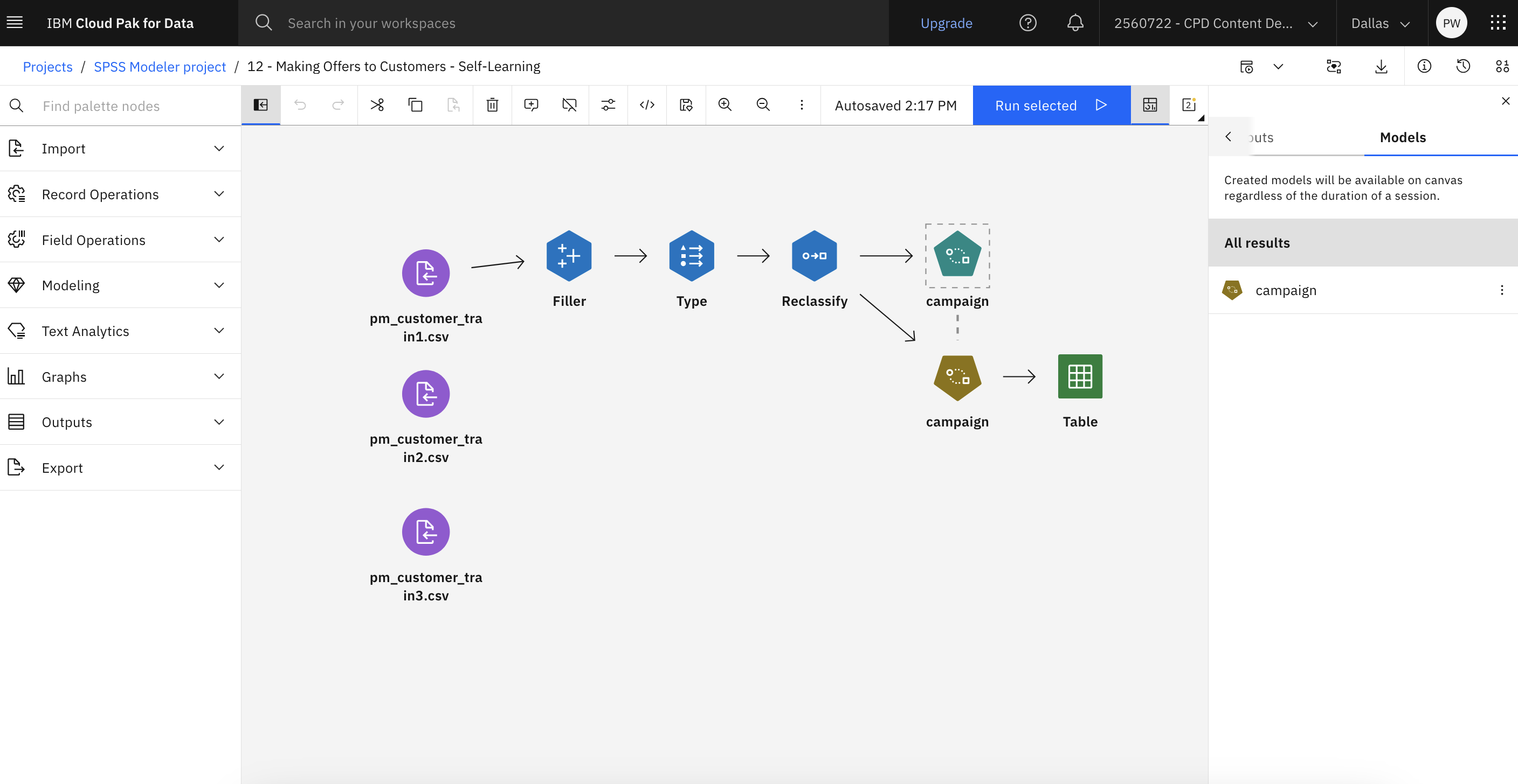
- In the Outputs and models pane, click the campaign model to view the results.
The initial view shows the estimated accuracy of the predictions for each offer. You can also click Predictor Importance to see the relative importance of each predictor in estimating the model, or click Association With Response to show the correlation of each predictor with the target variable.
Figure 4. Campaign model performance 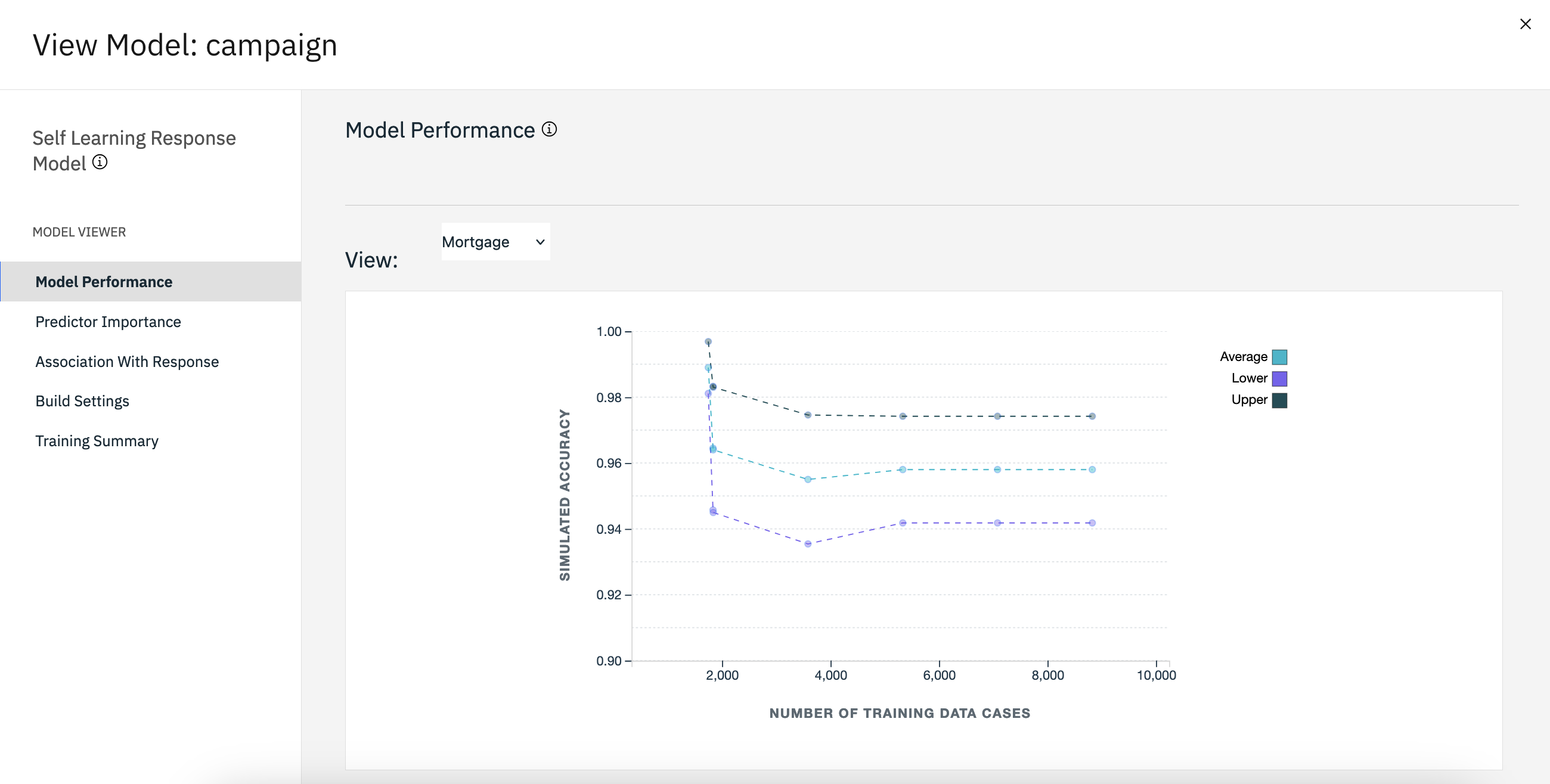
- To switch between each of the four offers for which there are predictions, use the View menu.
- Return to the flow.
Check your progress
The following image shows the flow. You are now ready to experiment with other Data Asset nodes.
Task 6: Experiment with other Data Asset nodes
Follow these steps to experiment with other Data Asset nodes:
- Disconnect the pm_customer_train1.csv node from the Filler node.
- Connect the pm_customer_train2.csv node to the Filler node.
- Double-click the campaign (SLRM) node, and under the Build Options make sure that Continue training existing model is selected.
- Click Save.
- Run the flow to regenerate the model nugget. Hover over the campaign (SLRM) node, and
click the Run icon
.
- In the Outputs and models pane, click the campaign model to view the results. The
model now shows the revised estimates of accuracy of the predictions for each offer.
Figure 5. Campaign model performance 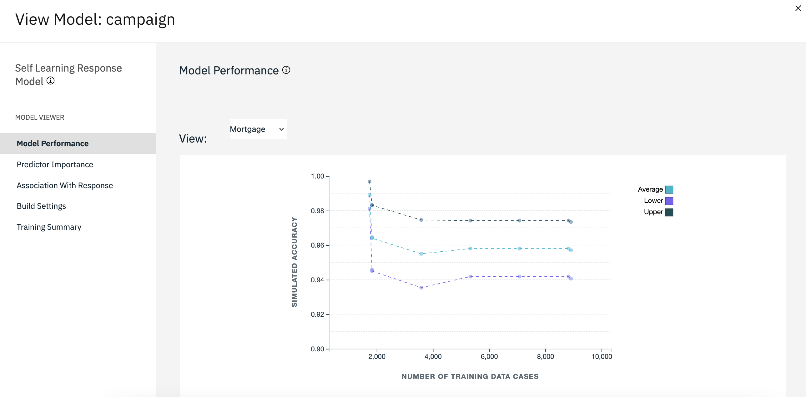
- Disconnect the pm_customer_train2.csv node from the Filler node.
- Connect the pm_customer_train3.csv node to the Filler node.
- Run the flow to regenerate the model nugget. Hover over the campaign (SLRM) node, and
click the Run icon
.
- In the Outputs and models pane, click the campaign model to view the results.
Figure 6. Campaign model performance 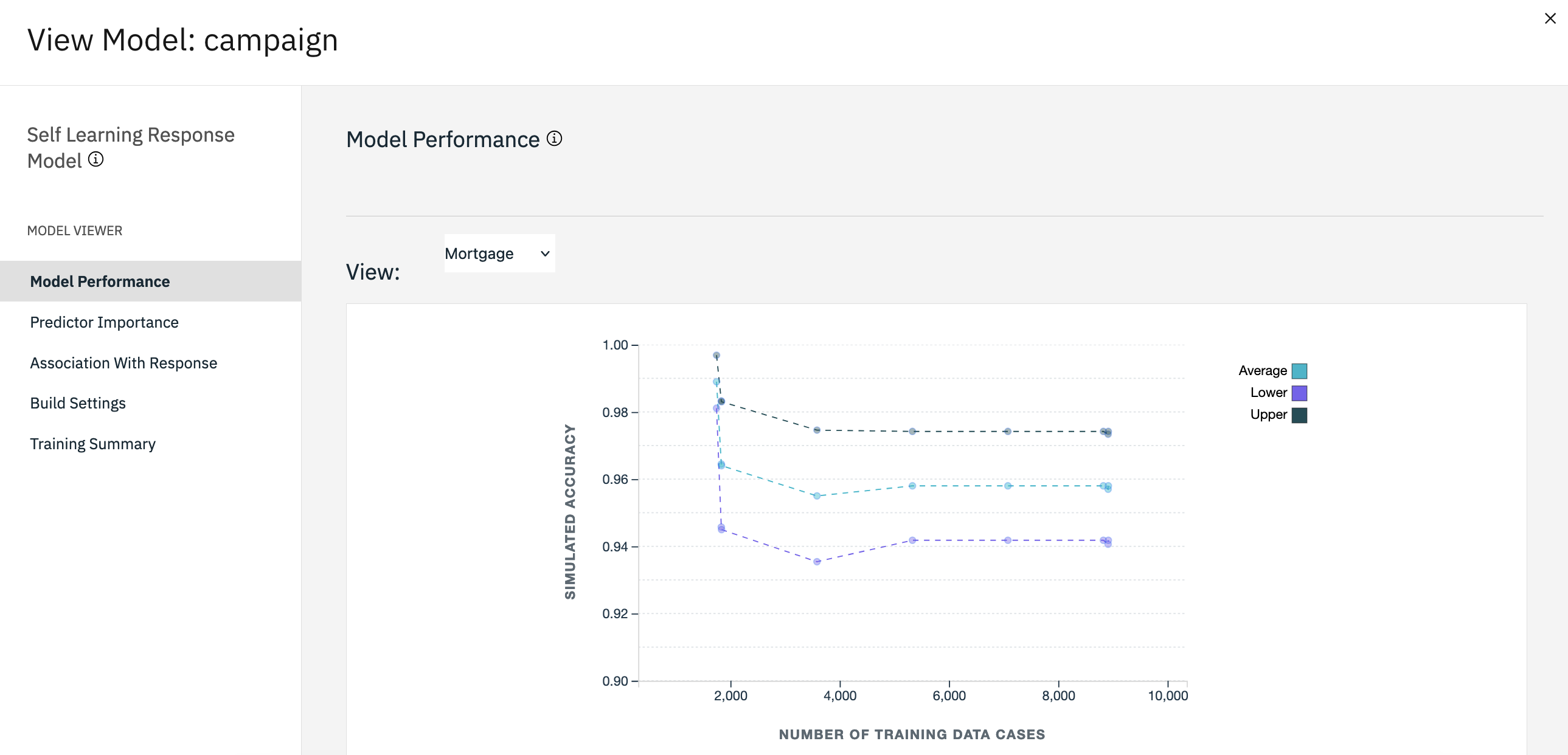
The model now shows the final estimated accuracy of the predictions for each offer. As you can see, the average accuracy fell slightly as you added the additional data sources. However, this fluctuation is a minimal amount and might be attributed to slight anomalies within the available data.
- Hover over the Table node, and click the Run icon
.
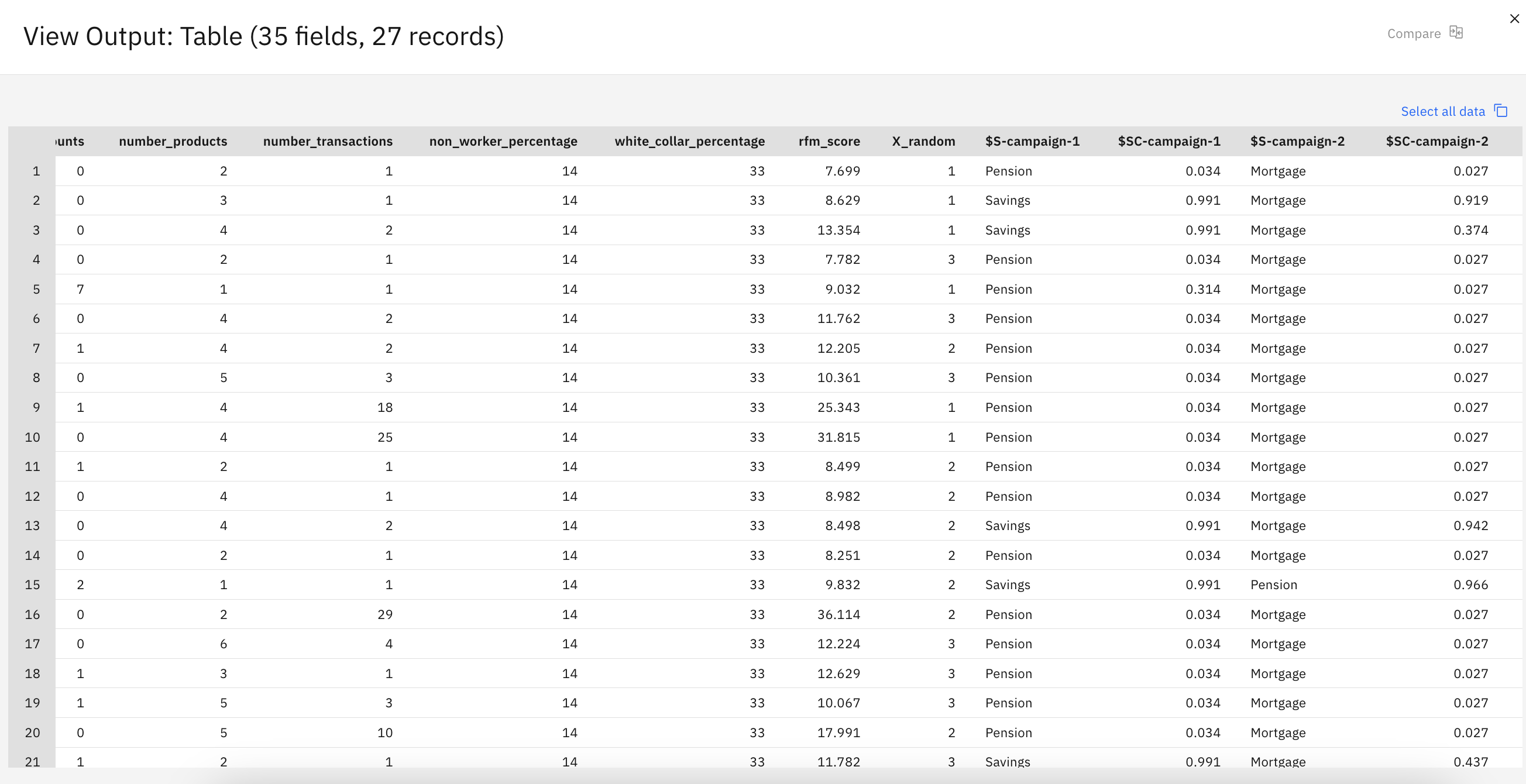
- In the Outputs and models pane, click the Table model to view the results.
Figure 7. Campaign model performance 
The predictions in the table show which offers a customer is most likely to accept and the
confidence that they accept that offer, depending on each customer's details. For example, in the
first row, there is only a 13.2% confidence rating (denoted by the value 0.132 in
the $SC-campaign-1 column) that a customer who previously took out a car loan
accepts a pension if offered one. However, the second and third lines show two more customers who
also took out a car loan; in their cases, there is a 95.7% confidence that they, and other customers
with similar histories, open a savings account if offered one, and over 80% confidence that they
accept a pension.
Explanations of the mathematical foundations of the modeling methods that are used in SPSS Modeler are available in the SPSS Modeler Algorithms Guide.
These results are based on the training data only. To assess how well the model generalizes to other data in the real world, you use a Partition node to hold out a subset of records for purposes of testing and validation.
Check your progress
The following image shows the flow.

Summary
This example showed how to use the Self-Learning Response Model (SLRM) node to predict which offers a customer is most likely to accept and the confidence that they accept the offer, depending on each customer's details.
Next steps
You are now ready to try other SPSS® Modeler tutorials.