This tutorial builds two models to predict the effects of future sales promotions, and then compares the models.
Similar to the Condition monitoring tutorial, the data
mining process consists of the exploration, data preparation, training, and test phases. Not all of
the data in the telco.csv data file are useful in predicting churn. You can use the
filter to select only data that is considered to be important for use as a predictor (the fields
marked as Important in the model).
Try the tutorial
In this tutorial, you will complete these tasks:
Sample modeler flow and data set
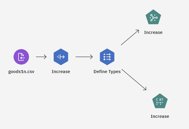
This tutorial uses the Retail Sales Promotion flow in the sample project. The data file used is goods2n.csv. The following image shows the sample modeler flow.


Task 1: Open the sample project
The sample project contains several data sets and sample modeler flows. If you don't already have the sample project, then refer to the Tutorials topic to create the sample project. Then follow these steps to open the sample project:
- In Cloud Pak for Data, from the Navigation menu
, choose Projects > View all Projects.
- Click SPSS Modeler Project.
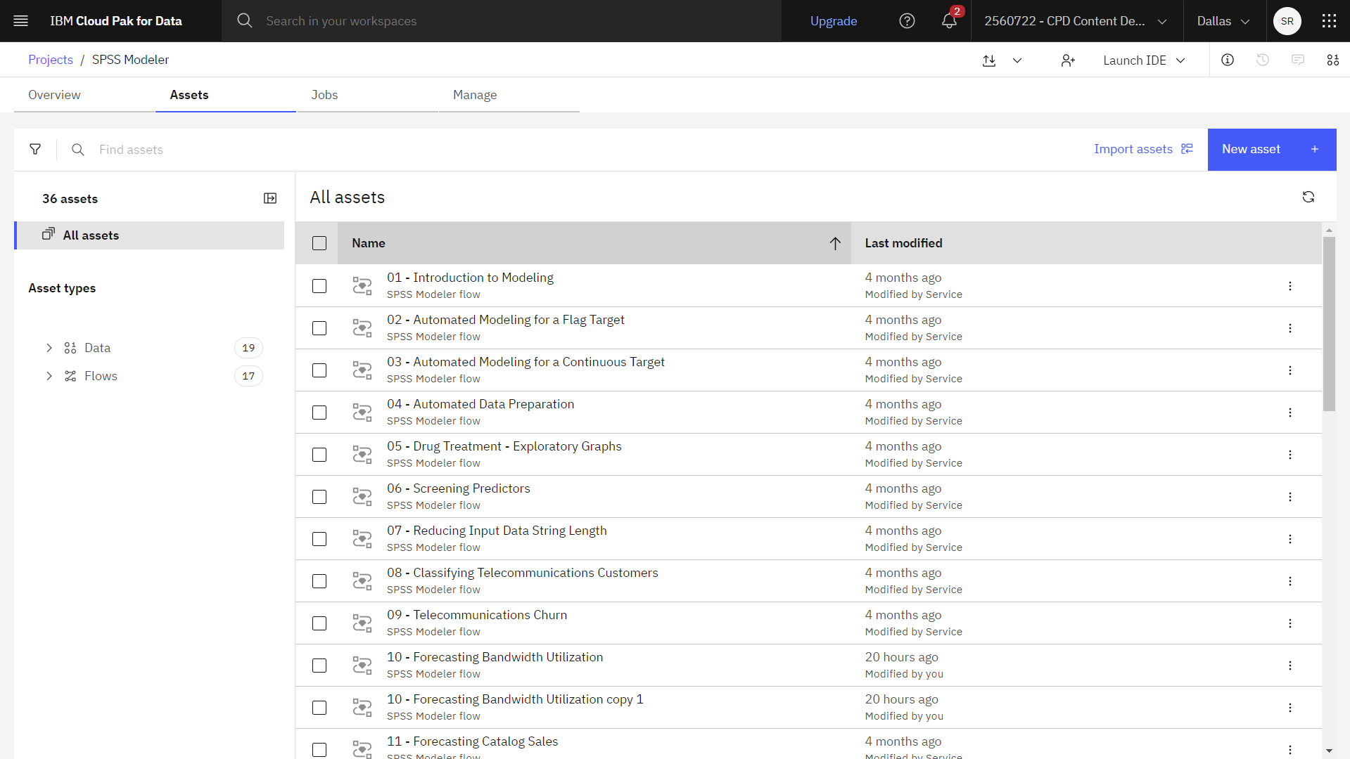
- Click the Assets tab to see the data sets and modeler flows.
Check your progress
The following image shows the project Assets tab. You are now ready to work with the sample modeler flow associated with this tutorial.

Task 2: Examine the Data Asset, Derive, and Type nodes
Retail Sales Promotion includes several nodes. Follow these steps to examine the Data Asset, Derive, and Type nodes:
Data Asset node
- From the Assets tab, open the Retail Sales Promotion modeler flow, and wait for the canvas to load.
- Double-click the goods1n.csv node. This node is a Data Asset node that points to the goods1n.csv file in the project.
- Review the File format properties.
- Click Preview data to see the full data set.
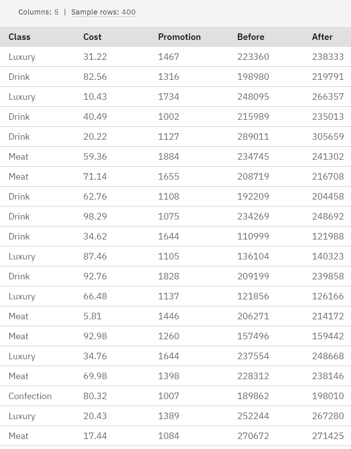
- Notice that each record contains:
Class. Product type.Cost. Unit price.Promotion. Index of amount spent on a particular promotion.Before. Revenue before promotion.After. Revenue after promotion.
The two revenue fields (
BeforeandAfter) are expressed in absolute terms. However, it seems likely that the increase in revenue after the promotion (and presumably as a result of it) might be a more useful figure. - Close the data preview and the properties side pane.
Derive node
- Double-click the Increase (Derive) node. This node derives the value of the increase in revenue.
- Review the settings, in particular, the Expression field; which contains a formula to
derive the increase as a percentage of the revenue before the promotion:
(After - Before) /
Before * 100.0
. - Click Preview data to see the data set with the derived values.
- Notice the Increase column.
For each class of product, and almost linear relationship exists between the increase in revenue and the cost of the promotion. Therefore, it seems likely that a decision tree or neural network could predict, with reasonable accuracy, the increase in revenue from the other available fields.
- Close the data preview and the properties side pane.
Type node
- Double-click the Define Types (Type) node. This node specifies field properties, such as
measurement level (the type of data that the field contains), and the role of each field as a target
or input in modeling. The measurement level is a category that indicates the type of data in the
field. The source data file uses three different measurement levels:
- A Continuous field (such as the
Agefield) contains continuous numeric values. - A Nominal field (such as the
Educationfield) has two or more distinct values—in this caseCollegeorHigh school. - An Ordinal field (such as the
Income levelfield) describes data with multiple distinct values that have an inherent order—in this caseLow,Medium, andHigh.For each field, the Type node also specifies a role to indicate the part that each field plays in modeling. The role is set to Target for the field
Increase, which is the field that was derived. Thetargetis the field for which you want to predict the value.Role is set to Input for most other fields. Input fields are sometimes known as
predictors, or fields whose values are used by the modeling algorithm to predict the value of the target field.The role for the
Afterfield is set to None, so this field is not used by the modeling algorithm.
- A Continuous field (such as the
- Optional: Click Preview data to see the data set with the derived values.
Check your progress
The following image shows the Type node. You are now ready to generate and compare the models.

Task 3: Generate and compare the models
The flow trains a neural network and a decision tree to make this prediction of revenue increase. Follow these steps to generate the two models:
Generate the models
- Double-click the Increase (Neural net) node to review its properties.
- Expand the Basics section to see that the Multilayer Perceptron is the model type. This property determines how the network connects the predictors to the targets through the hidden layers. Multilayer perceptron allows for more complex relationships at the possible cost of increasing the training and scoring time.
- Expand the Model Options section to see the evaluation and scoring properties.
- Double-click the Increase (C&R Tree) node to see its properties.
- Click Run all
, and wait for the model nuggets to generate.
- Connect the Increase (C&R Tree) model nugget to the Increase (Neural net).
- Add an Analysis node:
- From the palette, expand the Outputs section.
- Drag the Analysis node on to the canvas.
- Connect the Increase (Neural net) model nugget to the Analysis node.
- Change the data set to use different data for the analysis:
- Double-click the goods1n.csv node to view its properties.
- CV lick Change data set.
- Navigate to Data asset > GOODS2n.csv.
- Click Select.
- Click Save.
- Hover over the Analysis node, and click the Run icon
.
- In the Outputs and models pane, click the output with the name Analysis to view
the results.
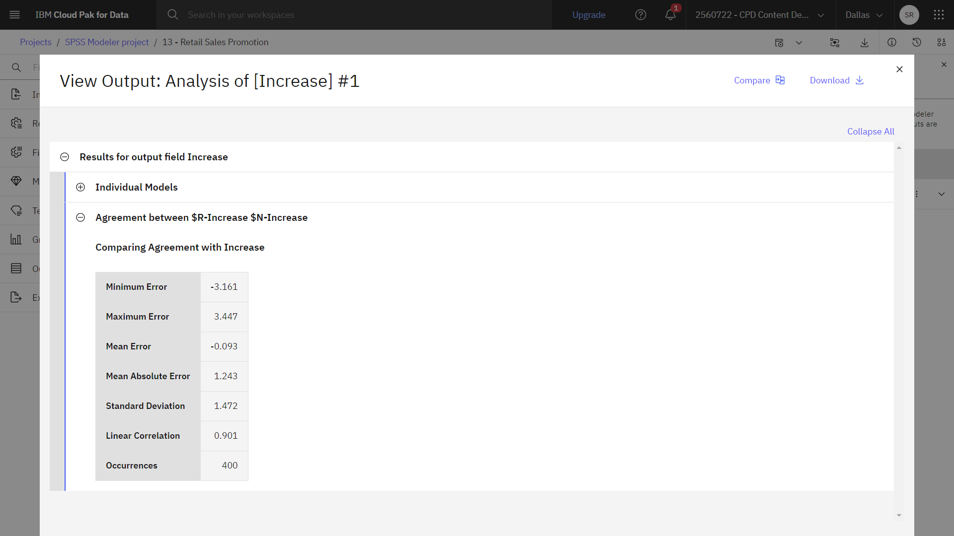
From the Analysis output, in particular from the linear correlation between the predicted increase and the correct answer, you see that the trained systems predict the increase in revenue with a high degree of success.
Further exploration might focus on the cases where the trained systems make relatively large errors. You might identify these errors by plotting the predicted increase in revenue against the actual increase. You might then select outliers on a graph by using the interactive graphics within SPSS Modeler, and from their properties, it might be possible to tune the data description or learning process to improve accuracy.
Check your progress
The following image shows the output from the Analysis node.

Summary
This example showed you how to predict the effects of future sales promotions. Similar to the condition monitoring example, the data mining process consists of the exploration, data preparation, training, and test phases.
Next steps
You are now ready to try other SPSS® Modeler tutorials.