Preview the tutorial
 Watch this video to preview the steps in this tutorial. There might
be slight differences in the user interface that is shown in the video. The video is intended to be
a companion to the written tutorial. This video provides a visual method to learn the concepts and
tasks in this documentation.
Try the tutorial
In this tutorial, you will complete these tasks:
Sample modeler flow and data set
This tutorial uses the Introduction to Modeling flow in the sample project. The data file used is tree_credit.csv. The following image shows the sample modeler flow.

The ability to predict an outcome is the central goal of predictive analytics, and understanding the modeling process is the key to using SPSS Modeler flows.
The model in this example shows how a bank can predict if future loan applicants might default on their loans. These customers previously took loans from the bank, so the customers’ data is stored in the bank's database. The model uses the customers’ data to determine how likely they are to default.
An important part of any model is the data that goes into it. The bank maintains a database of historical information on customers, including whether they repaid the loans (Credit rating = Good) or defaulted (Credit rating = Bad). The bank wants to use this existing data to build the model. The following fields are used:
| Field name | Description |
|---|---|
| Credit_rating | Credit rating: 0=Bad, 1=Good, 9=missing values |
| Age | Age in years |
| Income | Income level: 1=Low, 2=Medium, 3=High |
| Credit_cards | Number of credit cards held: 1=Less than five, 2=Five or more |
| Education | Level of education: 1=High school, 2=College |
| Car_loans | Number of car loans taken out: 1=None or one, 2=More than two |
This example uses a decision tree model, which classifies records (and predicts a response) by using a series of decision rules.

For example, this decision rule classifies a record as having a good credit rating when the income falls in the medium range and the number of credit cards are less than 5.
IF income = Medium
AND cards <5
THEN -> 'Good'
Using a decision tree model, you can analyze the characteristics of the two groups of customers and predict the likelihood of loan defaults.
While this example uses a CHAID (Chi-squared Automatic Interaction Detection) model, it is intended as a general introduction, and most of the concepts apply broadly to other modeling types in SPSS Modeler.
Task 1: Open the sample project
The sample project contains several data sets and sample modeler flows. If you don't already have the sample project, then refer to the Tutorials topic to create the sample project. Then follow these steps to open the sample project:
- In Cloud Pak for Data, from the Navigation menu
, choose Projects > View all Projects.
- Click SPSS Modeler Project.
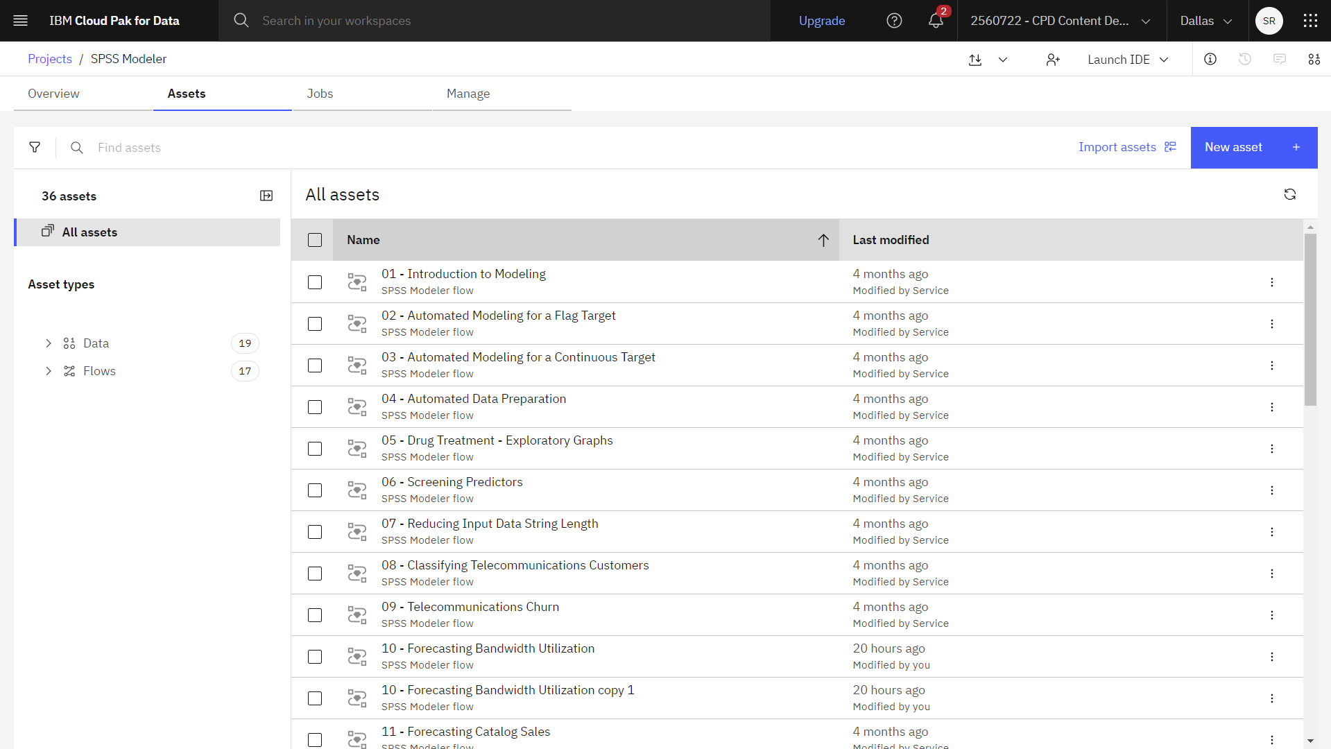
- Click the Assets tab to see the data sets and modeler flows.
Check your progress
The following image shows the project Assets tab. You are now ready to work with the sample modeler flow associated with this tutorial.
Task 2: Examine the Data Asset and Type nodes
Introduction to Modeling modeler flow includes several nodes. Follow these steps to examine the Data Asset and Type nodes.
- From the Assets tab, open the Introduction to Modeling modeler flow, and wait for the canvas to load.
- Double-click the tree_credit.csv node. This node is a Data Asset node that points to the tree_credit.csv file in the project. If you specify measurements in the source node, you don’t need to include a separate Type node in the flow.
- Review the File format properties.
- Optional: Click Preview data to see the full data set.
- Double-click the Type node. This node specifies field properties, such as measurement
level (the type of data that the field contains), and the role of each field as a target or input in
modeling. The measurement level is a category that indicates the type of data in the field. The
source data file uses three different measurement levels:
- A Continuous field (such as the
Agefield) contains continuous numeric values. - A Nominal field (such as the
Educationfield) has two or more distinct values: in this case,CollegeorHigh school. - An Ordinal field (such as the
Income levelfield) describes data with multiple distinct values that have an inherent order: in this case,Low,Medium, andHigh.
Figure 3. Type node 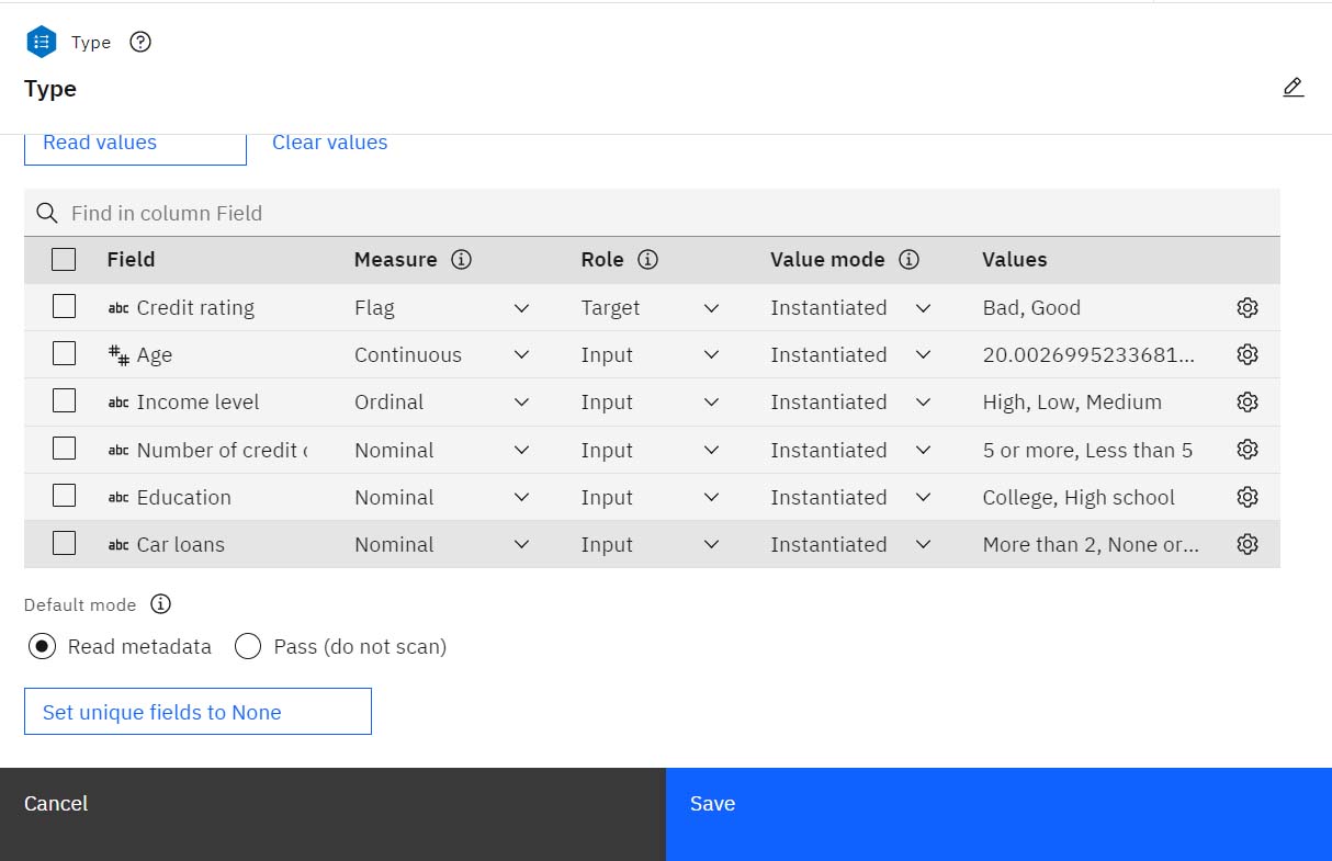
For each field, the Type node also specifies a role to indicate the part that each field plays in modeling. The role is set to Target for the field
Credit rating, which is the field that indicates whether a customer defaulted on the loan. The target is the field for which you want to predict the value.The other fields have the Role set to Input. Input fields are sometimes known as predictors, or fields whose values are used by the modeling algorithm to predict the value of the target field.
- A Continuous field (such as the
- Optional: Click Preview data to see the data with the Type properties applied.
Check your progress
The following image shows the Type node. You are now ready to configure the Modeling node.

Task 3: Configure the Modeling node
A modeling node generates a model nugget when the flow runs. This example uses a CHAID node. CHAID, or Chi-squared Automatic Interaction Detection, is a classification method that builds decision trees by using a particular type of statistics that are known as chi-square statistics. The node uses chi-square statistics to determine the best places to make the splits in the decision tree. Follow these steps to configure the Modeling node:
- Double-click the Credit rating (CHAID) node to see its properties.
- In the Fields section, notice the Use settings defined in this node option. This option tells the node to use the target and fields specified here instead of using the field information in the Type node. For this tutorial, leave the Use settings defined in this node option turned off.
- Expand the Objectives section. In this case, the default values are appropriate. Your objective is to Build new model, Create a standard model, and Generate a model node after run.
- Expand the Stopping Rules section. To keep the tree fairly simple for this example, limit
the tree growth by raising the minimum number of cases for parent and child nodes.
- Select Use absolute value.
- Set Minimum records in parent branch to
400. - Set Minimum records in child branch to
200.
- Click Save.
- Hover over the Credit rating (CHAID) node, and click the Run icon
.
Check your progress
The following image shows the flow with the model results. You are now ready to explore the model.

Task 4: Explore the model
Running the modeler flow adds a model nugget to the canvas with a link to the Modeling node from which it was created. Follow these steps to view the model details:
- In the Outputs and models pane, click the model with the name Credit rating to view the model.
- Click Model Information to see basic information about the model.
- Click Feature Importance to see the relative importance of each predictor in estimating
the model. From this chart, you can see that Income level is easily the most significant in
this case, with Number of credit cards as the next most significant factor.
Figure 4. Feature Importance chart 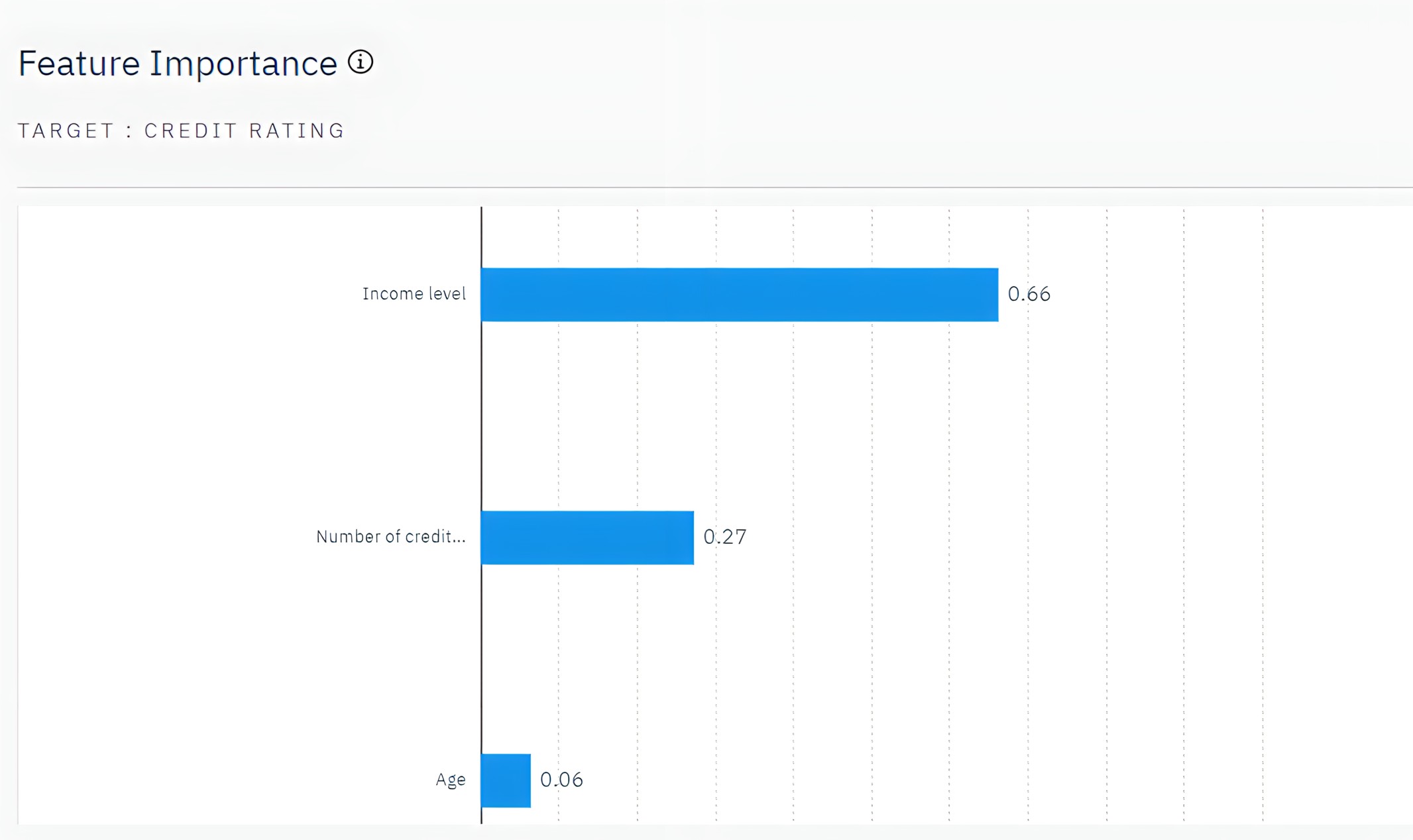
- Click Top Decision Rules to see details in the form of a rule set; essentially a series
of rules that can be used to assign individual records to child nodes based on the values of
different input fields. A prediction of Good or Bad is returned for each terminal node
in the decision tree. Terminal nodes are those tree nodes that are not split further. In each case,
the prediction is determined by the mode, or most common response, for records that fall within that
node.
Figure 5. CHAID model nugget, rule set 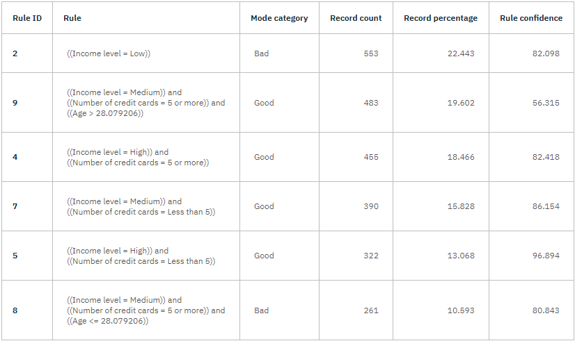
- Click Tree Diagram to see the same model in the form of a tree, with a node at each
decision point. Hover over branches and nodes to explore details.
Figure 6. Tree diagram in the model nugget 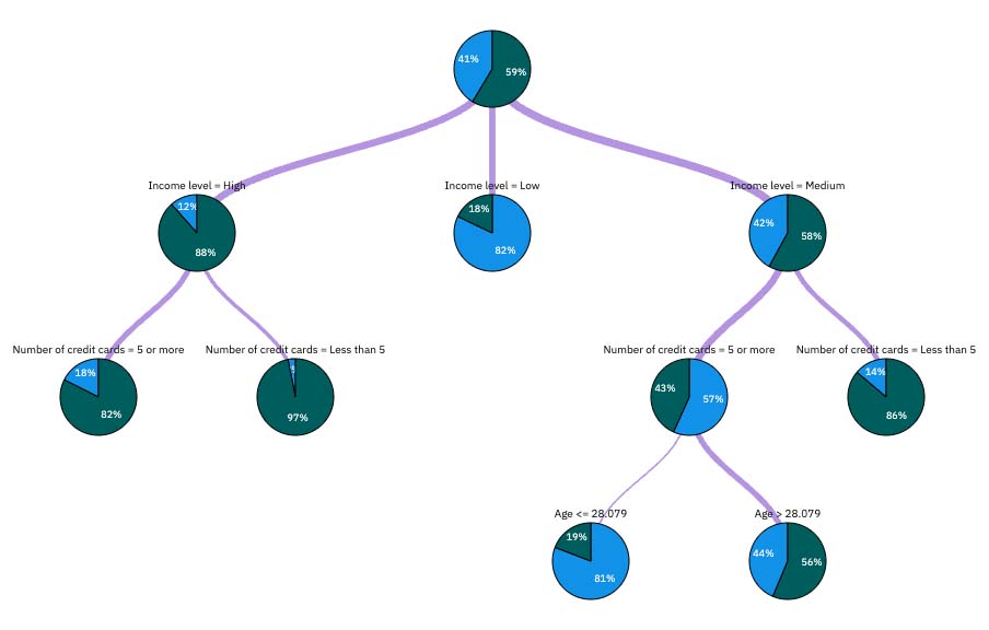
Looking at the start of the tree, the first node (node 0) gives a summary for all the records in the data set. Just over 40% of the cases in the data set are classified as a bad risk. 40% is quite a high proportion, but the tree might give clues as to what factors might be responsible.
The first split is by Income level. Records where the income level is in the Low category are assigned to node 2, and it's no surprise to see that this category contains the highest percentage of loan defaulters. Clearly, lending to customers in this category carries a high risk. However, almost 18% of the customers in this category didn’t default, so the prediction is not always correct. No model can feasibly predict every response, but a good model should allow you to predict the most likely response for each record based on the available data.
In the same way, if you look at the high-income customers (node 1), you can see that most customers (over 88%) are a good risk. But more than 1 in 10 of these customers still defaulted. Can the lending criteria be refined further to minimize the risk here?
Notice how the model divided these customers into two subcategories (nodes 4 and 5), based on the number of credit cards held. For high-income customers, if the bank lends to only customers with fewer than five credit cards, it can increase its success rate from 88% to almost 97%; an even more satisfactory outcome.
Figure 7. High-income customers with fewer than five credit cards 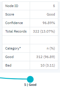
But what about those customers in the Medium income category (node 3)? They’re much more evenly divided between Good and Bad ratings. Again, the subcategories (nodes 6 and 7 in this case) can help. This time, lending only to those medium-income customers with fewer than five credit cards increases the percentage of Good ratings from 58% to 86%, a significant improvement.
Figure 8. Tree view of medium-income customers 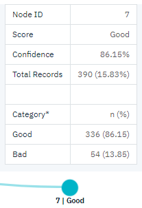
Check your progress
The following image shows the model details. You are now ready to evaluate the model.

Task 5: Evaluate the model
You can browse the model to understand how scoring works. However, to evaluate how accurately the model works, you need to score some records. Scoring records is the process of comparing the actual results to the responses that the model predicted. To evaluate the model, you can score the same records that were used to estimate the model. You can compare the observed and predicted responses by comparing the same records. Follow these steps to evaluate the model:
- Attach the Table node to the model nugget.
- Hover over the Table node, and click the Run icon
.
- In the Outputs and models pane, click the output results with the name Table to
view the results.
The table displays the predicted scores in the
$R-Credit ratingfield, which the model created. You can compare these values to the originalCredit ratingfield that contains the actual responses.By convention, the names of the fields that were generated during scoring are based on the target field, but with a standard prefix.$Gand$GEare prefixes for predictions that the Generalized Linear Model generates$Ris the prefix for predictions that the CHAID model generates$RCis for confidence values$Xis typically generated by using an ensemble$XR,$XS,$XFare used as prefixes in cases where the target field is a Continuous, Categorical, Set, or Flag field
A confidence value is the model's own estimation, on a scale from 0.0 to 1.0, of how accurate each predicted value is.
Figure 9. Table showing generated scores and confidence values 
As expected, the predicted value matches the actual responses for many records, but not all. The reason for this is that each CHAID terminal node has a mix of responses. The prediction matches the most common one, but it is wrong for all the others in that node. (Recall the 18% minority of low-income customers who did not default.)
To avoid this issue, you could continue splitting the tree into smaller and smaller branches until every node was 100% pure; all Good or Bad with no mixed responses. But such a model is complicated and is unlikely to generalize well to other data sets.
To find out exactly how many predictions are correct, you could read through the table and tally the number of records where the value of the predicted field
$R-Credit ratingmatches the value ofCredit rating. However, it is easiest to use an Analysis node, which automatically tracks records where these values match. - Connect the model nugget to the Analysis node.
- Hover over the Analysis node, and click the Run icon
.
- In the Outputs and models pane, click the output results with the name Analysis to
view the results.
The analysis shows that for 1960 out of 2464 records (over 79%) the value that the model predicted matched the actual response.
Figure 10. Analysis results comparing observed and predicted responses 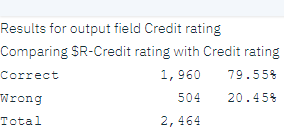
This result is limited by the fact that the records that you scored are the same ones that you used to estimate the model. In a real situation, you could use a Partition node to split the data into separate samples for training and evaluation. By using one sample partition to generate the model and another sample to test it, you can get a better indication of how well it generalizes to other data sets.
You can use the Analysis node to test the model against records for which you already know the actual result. The next stage illustrates how you can use the model to score records for which you don't know the outcome. For example, this data set might include people who are not currently customers of the bank, but who are prospective targets for a promotional mailing.
Check your progress
The following image shows the flow with the output results. You are now ready to score the model with new data.

Task 6: Score the model with new data
Earlier, you scored the records that were used to estimate the model so that you could evaluate how accurate the model was. This example scores a different set of records from the ones used to create the model. Evaluating accuracy is one of the goals of modeling with a target field. You study records for which you know the outcome to identify patterns so that you can predict outcomes that you don't yet know.
You can update the existing Data Asset or
Import node to point to a different data file. Or you can add a
Data Asset or Import node that reads in the data you
want to score. Either way, the new data set must contain the same input fields that are used by the
model (Age, Income level, Education, and so on),
but not the target field Credit rating.
Alternatively, you can add the model nugget to any flow that includes the expected input fields. Whether read from a file or a database, the source type does not matter if the field names and types match the ones that are used by the model.
Check your progress
The following image shows the completed flow.

Summary
The Introduction to Modeling example flow demonstrates the basic steps for creating, evaluating, and scoring a model.
- The Modeling node estimates the model by studying records for which the outcome is known, and creates a model nugget. This process is sometimes referred to as training the model.
- The model nugget can be added to any flow with the expected fields to score records. By scoring the records for which you already know the outcome (such as existing customers), you can evaluate how well it performs.
- After you're satisfied that the model performs acceptably, you can score new data (such as prospective customers) to predict how they will respond.
- The data used to train or estimate the model can be referred to as the analytical or historical data. The scoring data might also be referred to as the operational data.
Next steps
You are now ready to try other SPSS Modeler tutorials.