Building a best-fit exponential smoothing model involves determining the model type (whether the model needs to include trend, seasonality, or both) and then obtaining the best-fit parameters for the chosen model.

The plot of men's clothing sales over time suggested a model with both a linear trend component and a multiplicative seasonality component. This implies a Winters' model. First, however, we will explore a simple model (no trend and no seasonality) and then a Holt's model (incorporates linear trend but no seasonality). This will give you practice in identifying when a model is not a good fit to the data, an essential skill in successful model building.

We'll start with a simple exponential smoothing model.

1. Add a Time Series node and attach it to the Type node. Double-click the node to edit its properties.
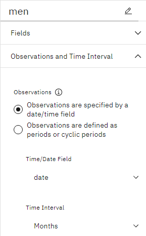
2. Under OBSERVATIONS AND TIME INTERVAL, select date as the time/date field.
3. Select Months as the time interval.

   

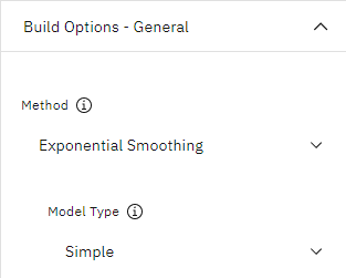
4. Under BUILD OPTIONS - GENERAL, select Exponential Smoothing for the Method.
5. Set Model Type to Simple. Click Save.

   

6. Run the flow to create the model nugget.
7. Attach a Time Plot node to the model nugget.
8. Under Plot, add the fields men and $TS-men to the Series list.
9. Select the option Use custom x axis field label and select the date field.
10. Deselect the Display series in separate panel and Normalize options. Click Save.

    

11. Run the flow and then open the output.
    The men plot represents the actual data, while $TS-men denotes the time series model.

    

    Although the simple model does, in fact, exhibit gradual (and rather ponderous) upward trend, it takes no account of seasonality. You can safely reject this model.

    Now let's try a Holt's linear model. This should at least model the trend better than the simple model, although it too is unlikely to capture the seasonality.

12. Double-click the Time Series node. Under BUILD OPTIONS - GENERAL, with Exponential Smoothing still selected as the method, select HoltsLinearTrend as the model type.
13. Click Save and run the flow again to regenerate the model nugget. Open the output.

    

    Holt's model displays a smoother upward trend than the simple model, but it still takes no account of the seasonality, so you can disregard this one too.

    You may recall that the initial plot of men's clothing sales over time suggested a model incorporating a linear trend and multiplicative seasonality. A more suitable candidate, therefore, might be Winters' model.

14. Double-click the Time Series node again to edit its properties.
15. Under BUILD OPTIONS - GENERAL, with Exponential Smoothing still selected as the method, select WintersMultiplicative as the model type.
16. Run the flow.

    

    This looks better. The model reflects both the trend and the seasonality of the data. The dataset covers a period of 10 years and includes 10 seasonal peaks occurring in December of each year. The 10 peaks present in the predicted results match up well with the 10 annual peaks in the real data.

    However, the results also underscore the limitations of the Exponential Smoothing procedure. Looking at both the upward and downward spikes, there is significant structure that's not accounted for.

    If you're primarily interested in modeling a long-term trend with seasonal variation, then exponential smoothing may be a good choice. To model a more complex structure such as this one, we need to consider using the ARIMA procedure.