About cookies on this site Our websites require some cookies to function properly (required). In addition, other cookies may be used with your consent to analyze site usage, improve the user experience and for advertising. For more information, please review your options. By visiting our website, you agree to our processing of information as described in IBM’sprivacy statement. To provide a smooth navigation, your cookie preferences will be shared across the IBM web domains listed here.
Last updated: Feb 12, 2025
This tutorial provides an example of how a medical researcher can compile and visual for
a study. The medical examiner collected data about a set of patients, all of whom suffered from the
same illness. During their course of treatment, each patient responded to one of five medications.
Part of your job is to use data mining to find out which drug might be appropriate for a future
patient with the same illness.
Preview the tutorial
 Watch this video to preview the steps in this tutorial. There might
be slight differences in the user interface that is shown in the video. The video is intended to be
a companion to the written tutorial. This video provides a visual method to learn the concepts and
tasks in this documentation.
Watch this video to preview the steps in this tutorial. There might
be slight differences in the user interface that is shown in the video. The video is intended to be
a companion to the written tutorial. This video provides a visual method to learn the concepts and
tasks in this documentation.
Try the tutorial
In this tutorial, you will complete these tasks:
- Task 1: Open the sample project
- Task 2: Examine the Data Asset
- Task 3: Explore the distribution and data audit charts
- Task 4: Create and explore the Scatter plot
- Task 5: Create and explore the web chart
- Task 6: Explore advanced visualizations
- Task 7: Explore the Derive node
- Task 8: Explore the Filter and Type nodes
- Task 9: Generate the model
- Task 10: Create an Analysis node
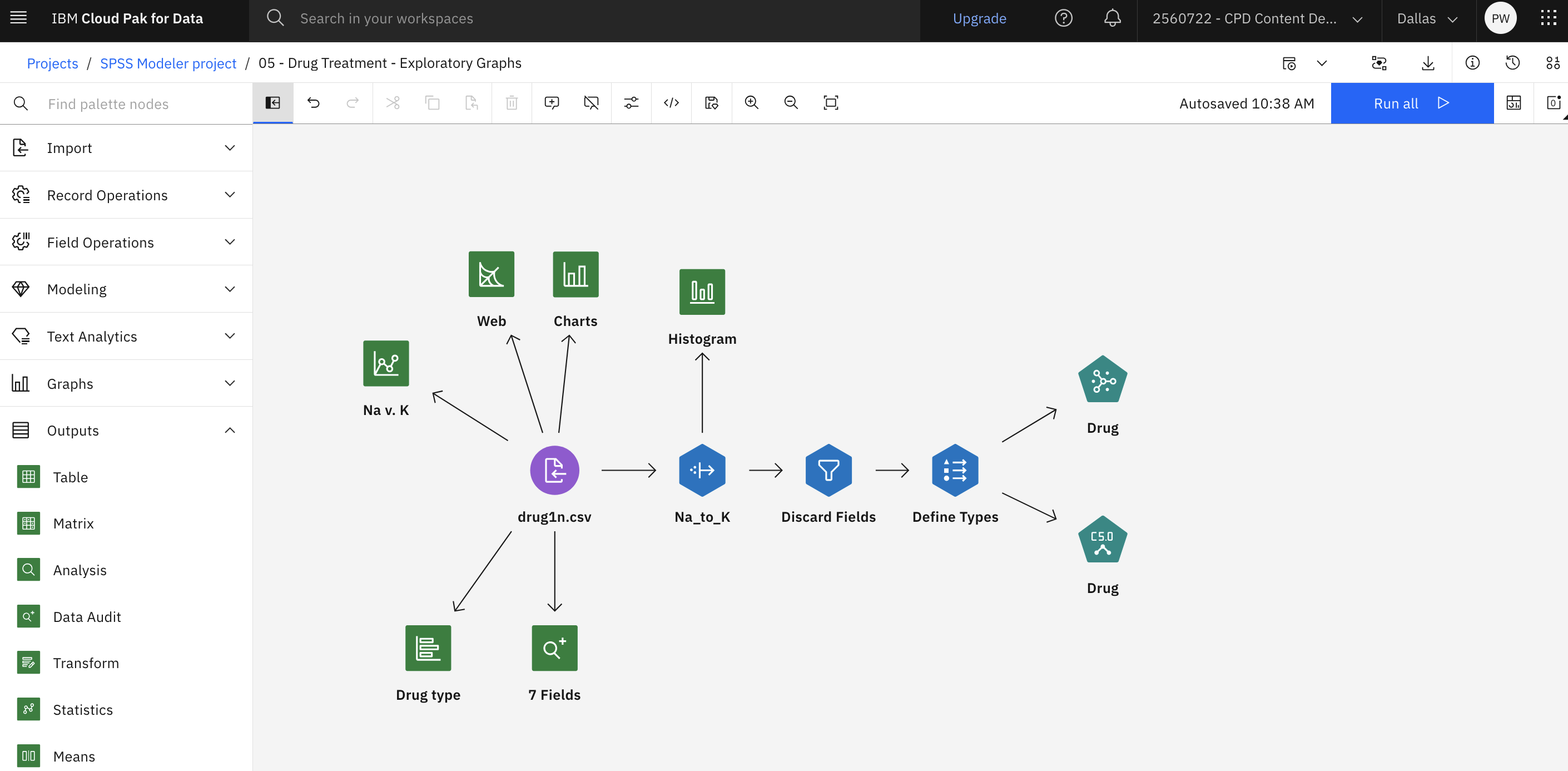
Sample modeler flow and data set
This tutorial uses the Drug Treatment - Exploratory Graphs flow in the sample project. The data file used is drug1n.csv. The following image shows the sample modeler flow.
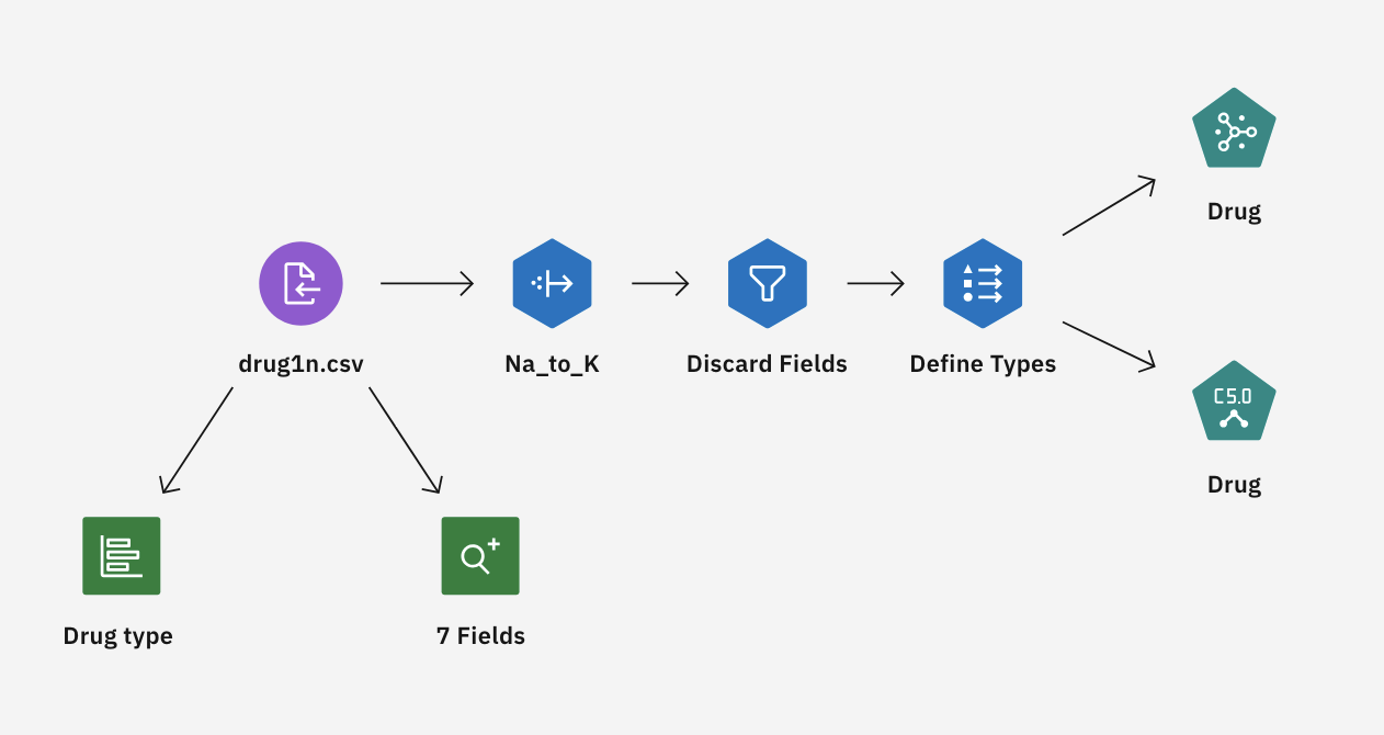
The data fields that are used in this example are:
| Data field | Description |
|---|---|
|
Age of patient (number) |
|
|
|
Blood pressure: |
|
Blood cholesterol: |
|
Blood sodium concentration |
|
Blood potassium concentration |
|
Prescription drug to which a patient responded |
Task 1: Open the sample project
The sample project contains several data sets and sample modeler flows. If you don't already have the sample project, then refer to the Tutorials topic to create the sample project. Then follow these steps to open the sample project:
- In watsonx, from the Navigation menu
 , choose
Projects > View all Projects.
, choose
Projects > View all Projects. - Click SPSS Modeler Project.
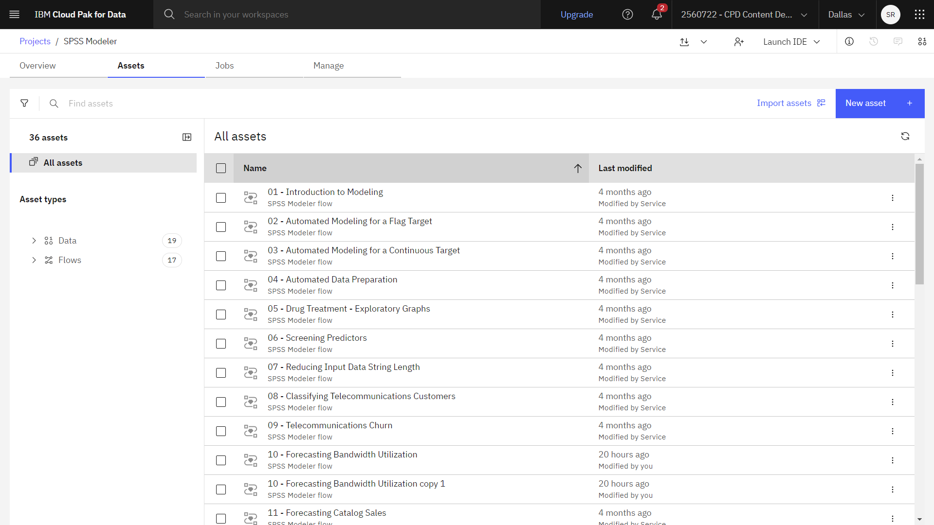
- Click the Assets tab to see the data sets and modeler flows.
![]() Check your progress
Check your progress
The following image shows the project Assets tab. You are now ready to work with the sample modeler flow associated with this tutorial.
Task 2: Examine the Data Asset
Drug Treatment - Exploratory Graphs includes several nodes. Follow these steps to examine the Data Asset node:
- From the Assets tab, open the Drug Treatment - Exploratory Graphs modeler flow, and wait for the canvas to load.
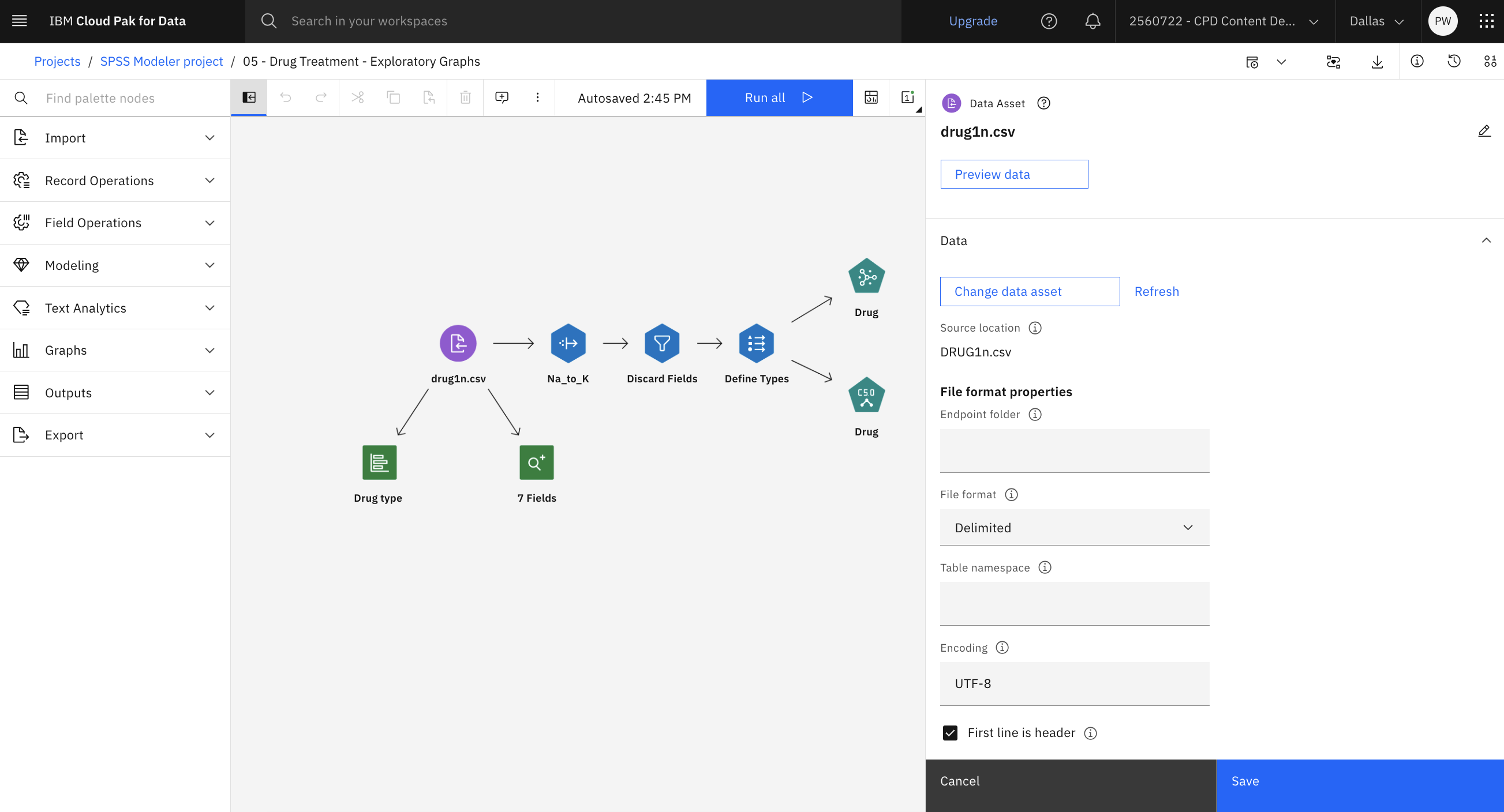
- Double-click the drug1n.csv node. This node is a Data Asset node that points to the drug1n.csv file in the project.
- Review the File format properties.
- Optional: Click Preview data to see the full data set.
![]() Check your progress
Check your progress
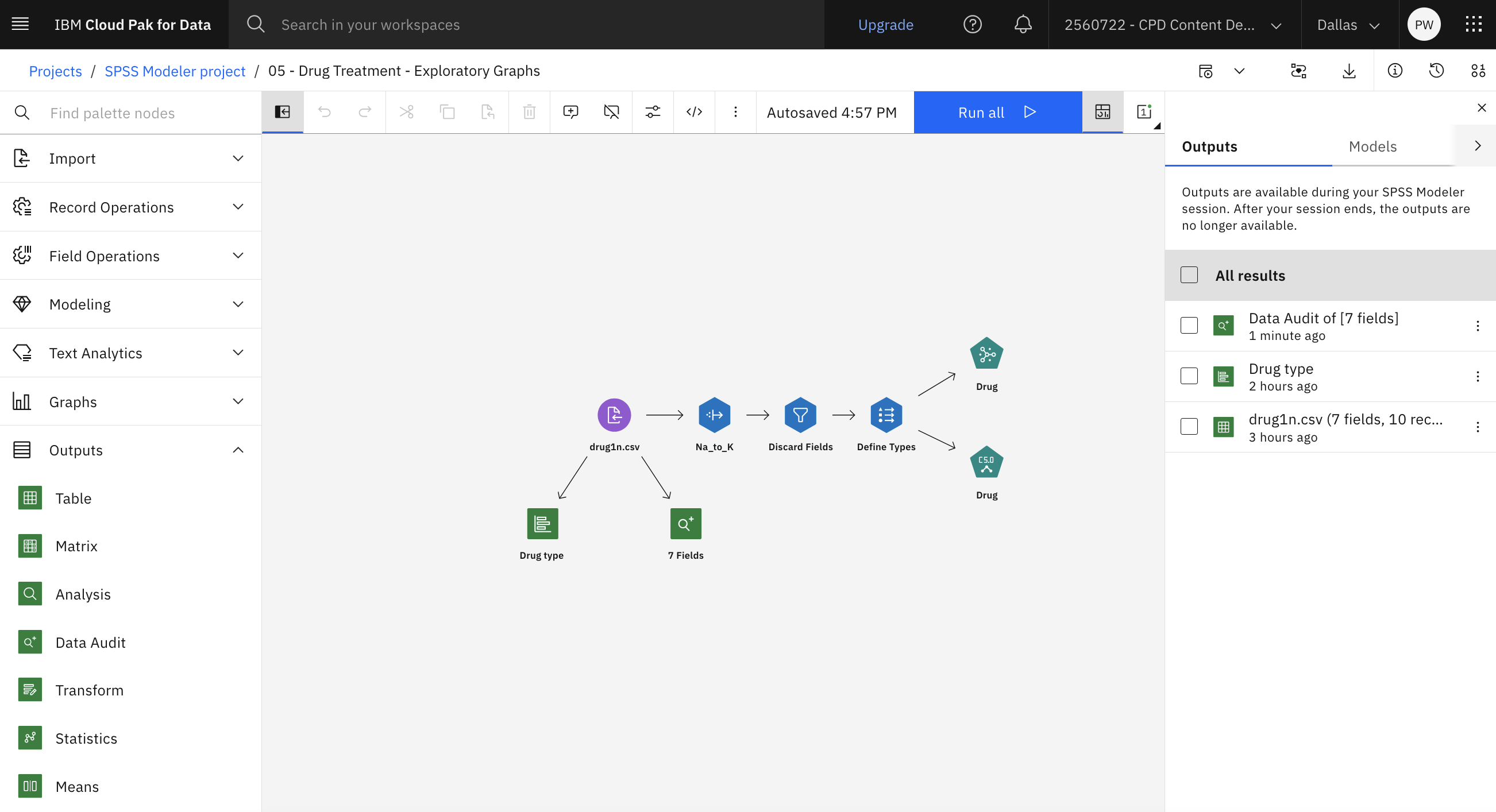
The following image shows the Data Asset node. You are now ready to explore the distribution and data audit charts.
Task 3: Explore the distribution and data audit charts
During data mining, it is often useful to explore the data by creating visual summaries. SPSS Modeler offers many different types of charts to choose from, depending on the type of data you want to summarize. For example, to find out what proportion of the patients responded to each drug, explore a Drug type (Distribution) node. Follow these steps to explore some charts:
- Double-click the Drug type (Distribution) node to see its properties.
- Click Cancel.
- Hover over the Drug type (Distribution) node and click the Run
icon
 .
. - In the Outputs and models pane, click the Drug type output to view the results.
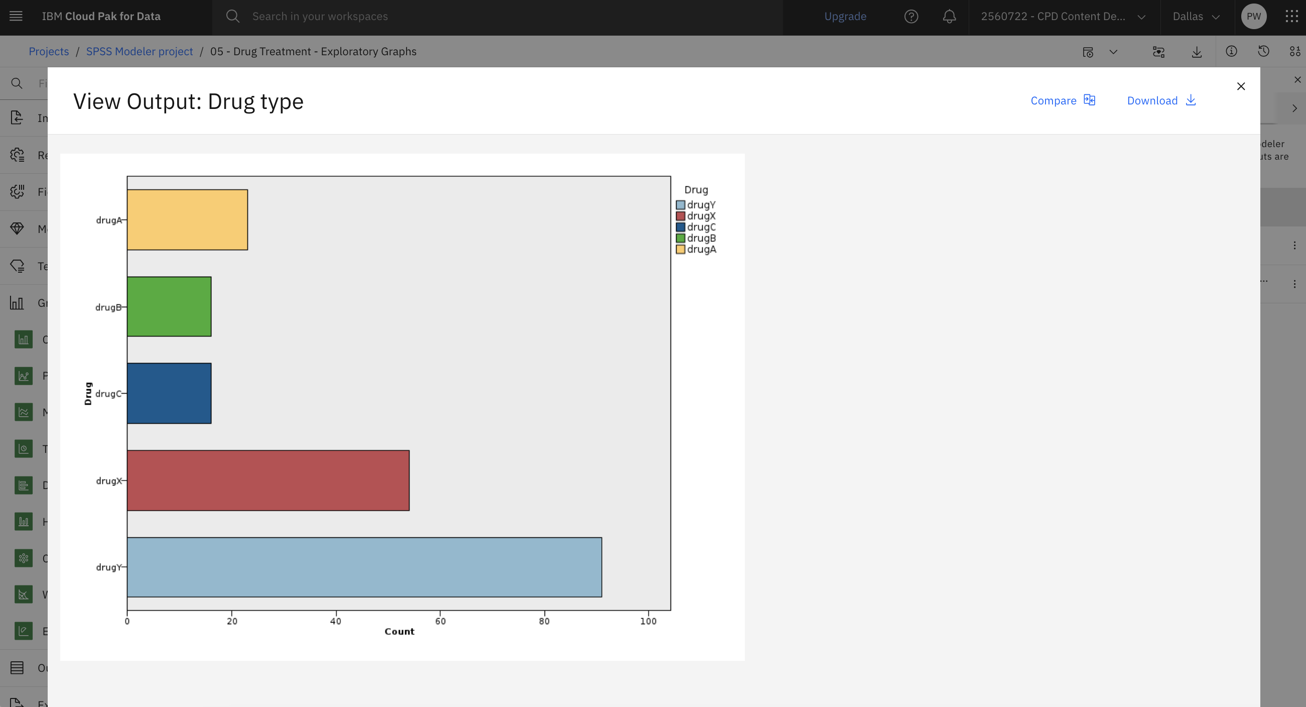
The chart helps you see the shape of the data. It shows that patients responded to
drug YBC
Alternatively, you can attach and run a 7 Fields (Data Audit) node to see distributions and histograms for all fields at once.
- Double-click the 7 Fields (Data Audit) output node after the Data Asset node.
- Hover over the 7 Fields (Data Audit) node and click the Run icon
.
- In the Outputs and models pane, click the 7 Fields (Data Audit) output to view the results.
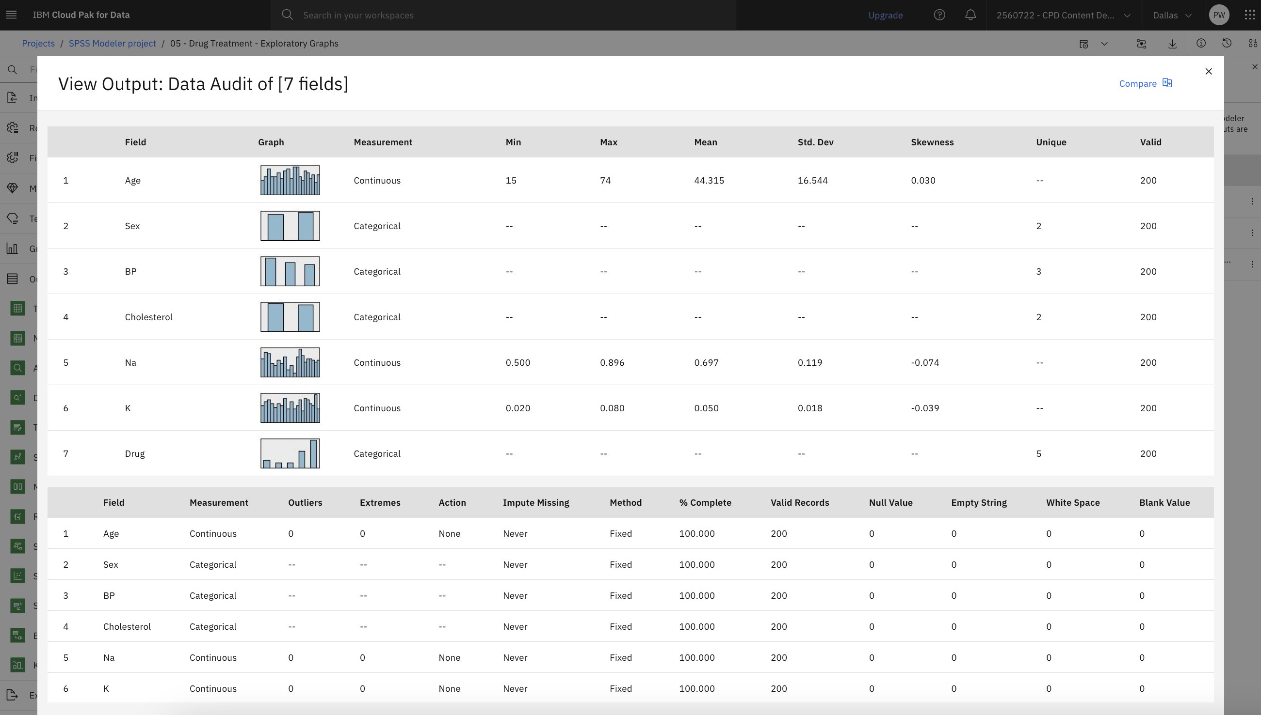
![]() Check your progress
Check your progress
The following image shows the flow. You are now ready to create and explore the Scatter plot.
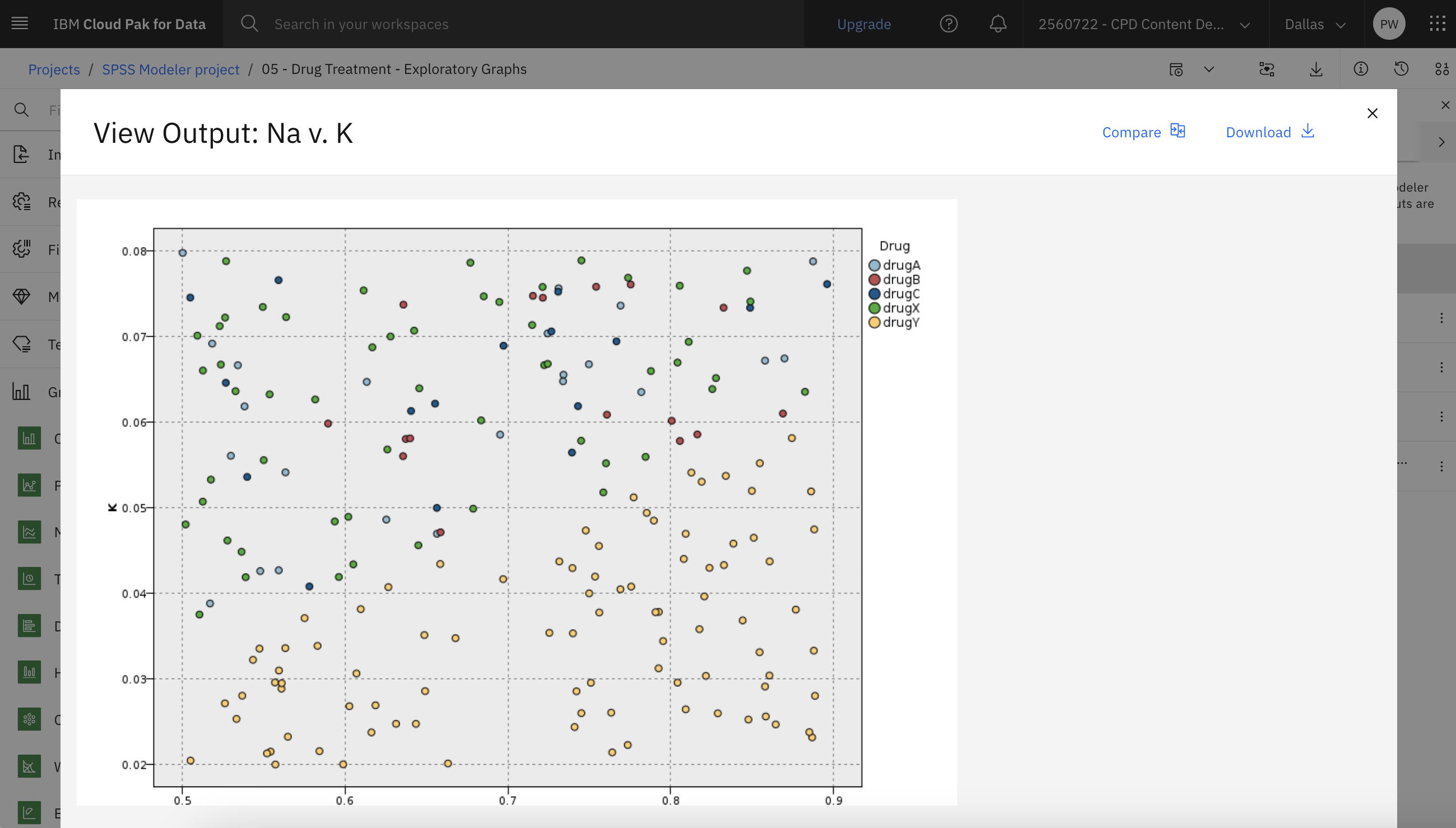
Task 4: Create and explore the Scatter plot
You can see what factors might influence Drug
- From the Graphs section in the palette, drag the Plot node onto the canvas.
- Hover over the node, click the Edit Title button, and rename it to Na v. K.
- Connect the Plot node to the drug1n.csv data asset node.
- Double-click the Na v. K (Plot) node to edit its properties.
- In the Plot section, select
NaKDrug - Click Save.
- Hover over the Na v. K (Plot) node and click the Run icon .
- In the Outputs and models pane, click the Na v. K output to view the results.
The plot clearly shows a threshold. For values higher than the threshold, drug YYNaK
![]() Check your progress
Check your progress
The following image shows the scatter plot. You are now ready to create and explore the web chart.
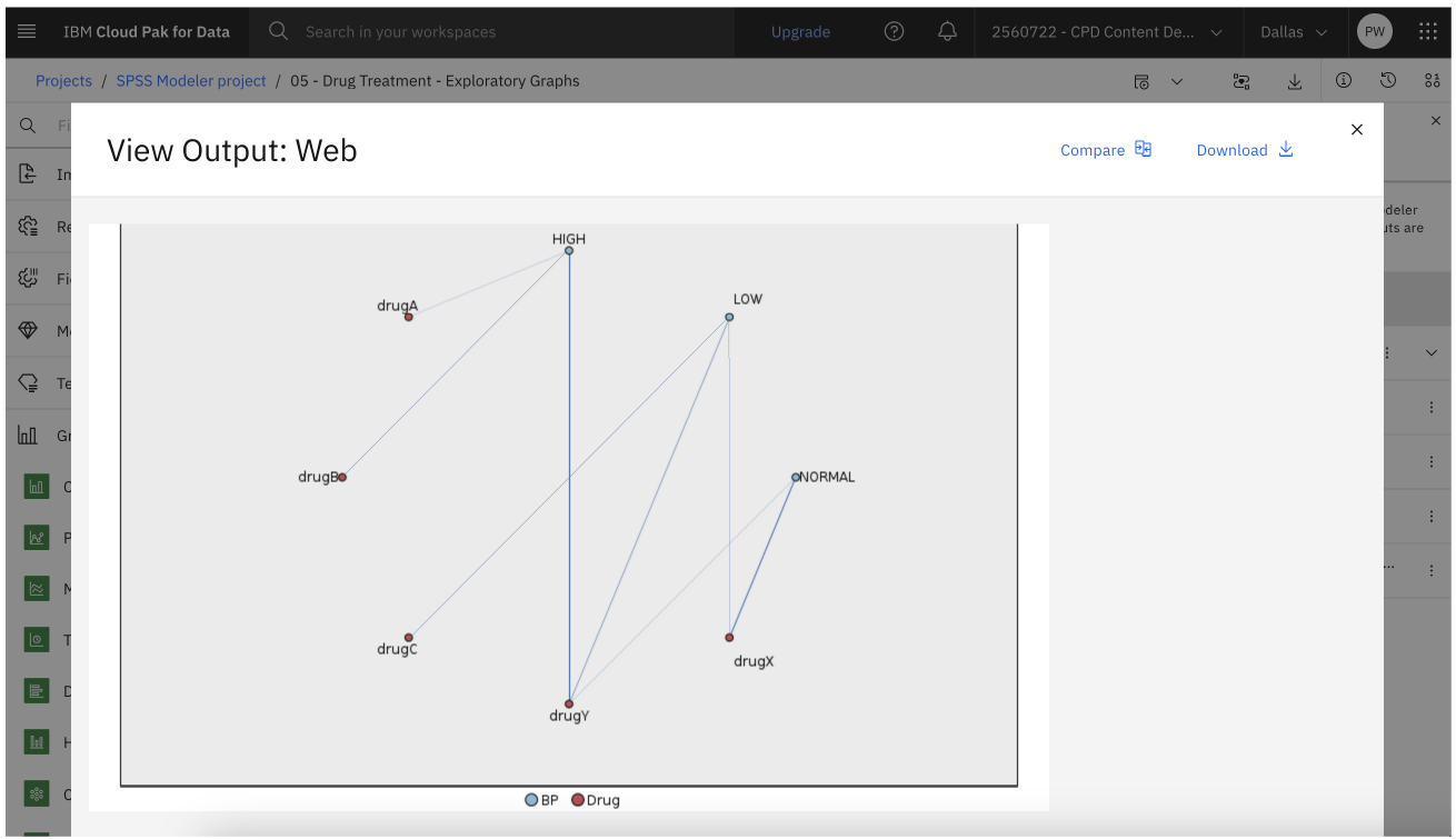
Task 5: Create and explore the web chart
Since many of the data fields are categorical, you can also try plotting a web chart, which maps associations between different categories. Follow these steps to explore a web chart:
- From the Graphs section in the palette, drag the Web node onto the canvas and connect it to the drug1n.csv data asset node.
- Double-click the Web node to edit its properties.
- In the Fields section, click Add columns. Select the
BPDrug - Click Save.
- Hover over the Web node and click the Run icon
- In the Outputs and models pane, click the Web output to view the results.
From the plot, apparently drug YY
But if you ignore drug YABCXXABCX
![]() Check your progress
Check your progress
The following image shows the web plot. You are now ready to explore advanced visualizations.
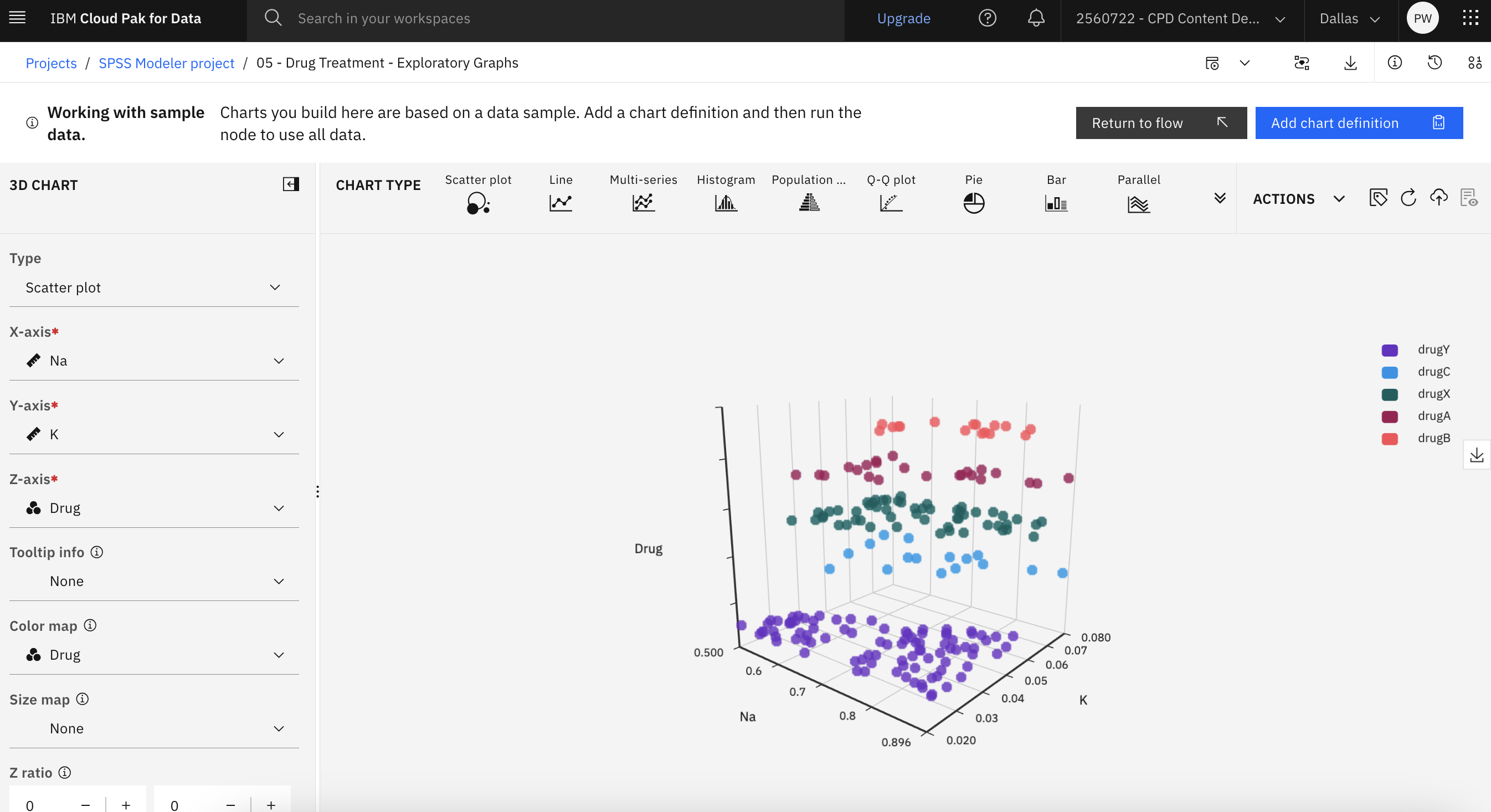
Task 6: Explore advanced visualizations
The previous sections use different types of graph nodes. Another way to explore data is with the advanced visualizations feature. Follow these steps to create and explore advanced charts:
- From the Graphs section in the palette, drag the Charts node onto the canvas and connect it to the drug1n.csv data asset node.
- Double-click the Charts node to see its properties.
- Click Launch Chart Builder button.
Here you can choose and create advanced charts to explore your data from different perspectives and identify patterns, connections, and relationships within your data. Experiment with creating some charts before you return to the modeler flow.
![]() Check your progress
Check your progress
The following image shows an example 3D chart. You are now ready to explore the Derive node.
Task 7: Explore the Derive node
As you saw with the scatter plot from Task 4, the ratio of sodium to potassium seems to predict when to use drug Y. You can derive a field that contains the value of this ratio for each record. This field might be useful later when you build a model to predict when to use each of the five drugs.
Follow these steps to explore the Derive node:
- Double-click the Na_to_K (Derive) node to edit its properties.
- Look at the Expression section. Na/K is the expression because you obtain the new
area by dividing the sodium value by the potassium value.
You can also create an expression by
clicking the calculator icon icon
 to open the Expression Builder; a way to interactively create expressions
by using built-in lists of functions, operands, and fields and their values.
to open the Expression Builder; a way to interactively create expressions
by using built-in lists of functions, operands, and fields and their values. - Click Cancel to return to the properties, and click Cancel again to return to the flow.
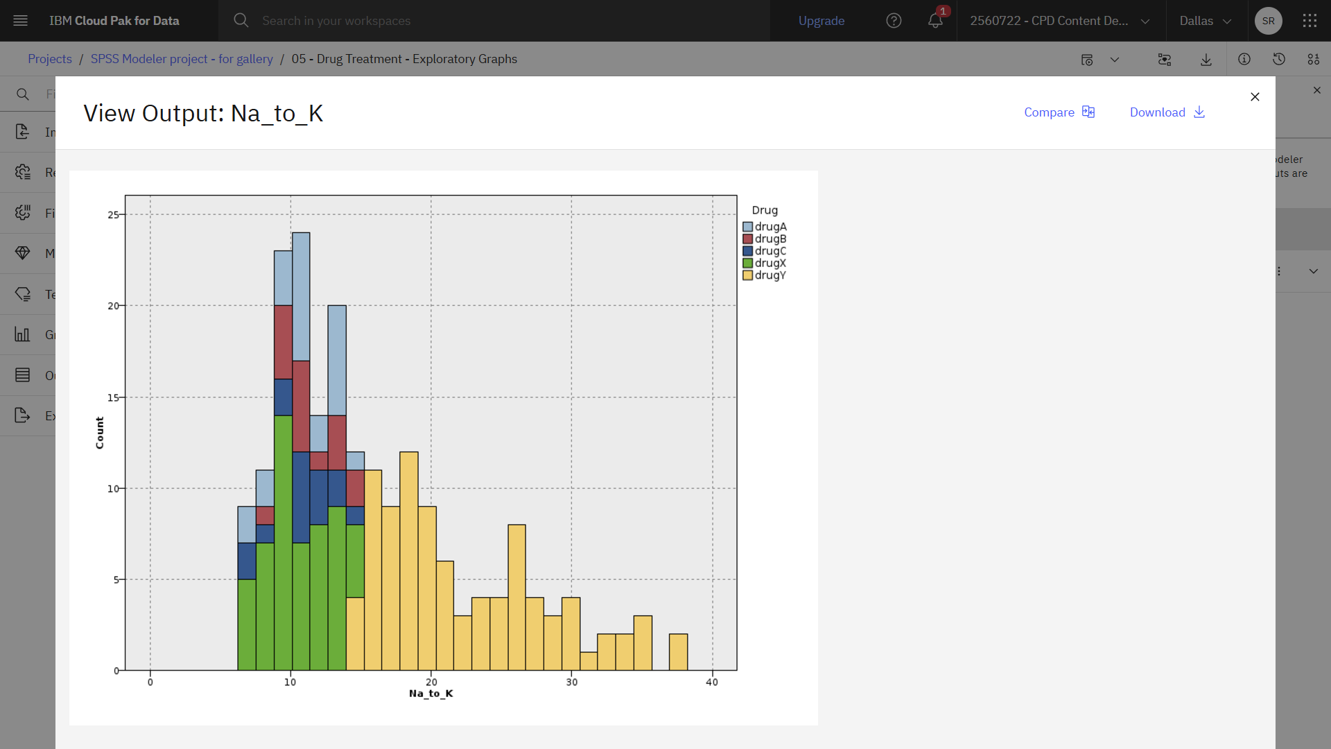
- From the Graphs section in the palette, drag the Histogram node onto the canvas and connect it to the Na_to_K (Derive) node.
- Double-click the Histogram node to see its properties.
- In the Histogram node properties, specify Na_to_K as the field to be plotted and Drug as the color overlay field.
- Click Save.
- Hover over the Histogram node, and click the Run icon .
- In the Outputs and models pane, click the Histogram output to view the results.
Based on the chart, you can conclude that when the Na_to_KY
![]() Check your progress
Check your progress
The following image shows the histogram. You are now ready to explore the Filter and Type nodes.
Task 8: Explore the Filter and Type nodes
By exploring and manipulating the data, you are able to form some hypotheses. The ratio of sodium to potassium in the blood seems to affect the choice of drug, as does blood pressure. But you cannot fully explain all of the relationships yet. Modeling can provide some answers. First, follow these steps to explore the Filter and Type nodes:
- Double-click the Discard Fields (Filter) node to see its properties.
- Since the derived field
Na_to_KNaKFigure 4. Filter node properties 
- Click Cancel.
- Double-click the Define Types (Type) node to see its properties.
- With the Type node, you can indicate the types of fields you're using and how they're
used to predict the outcomes. Notice that the role for the
DrugDrugFigure 5. Type node properties 
- Click Cancel.
![]() Check your progress
Check your progress
The following image shows the flow. You are now ready to generate the model.
Task 9: Generate the model
Follow these steps to generate the model by using a C5.0 node:
- Hover over the Drug (C5.0) node and click the Run icon .
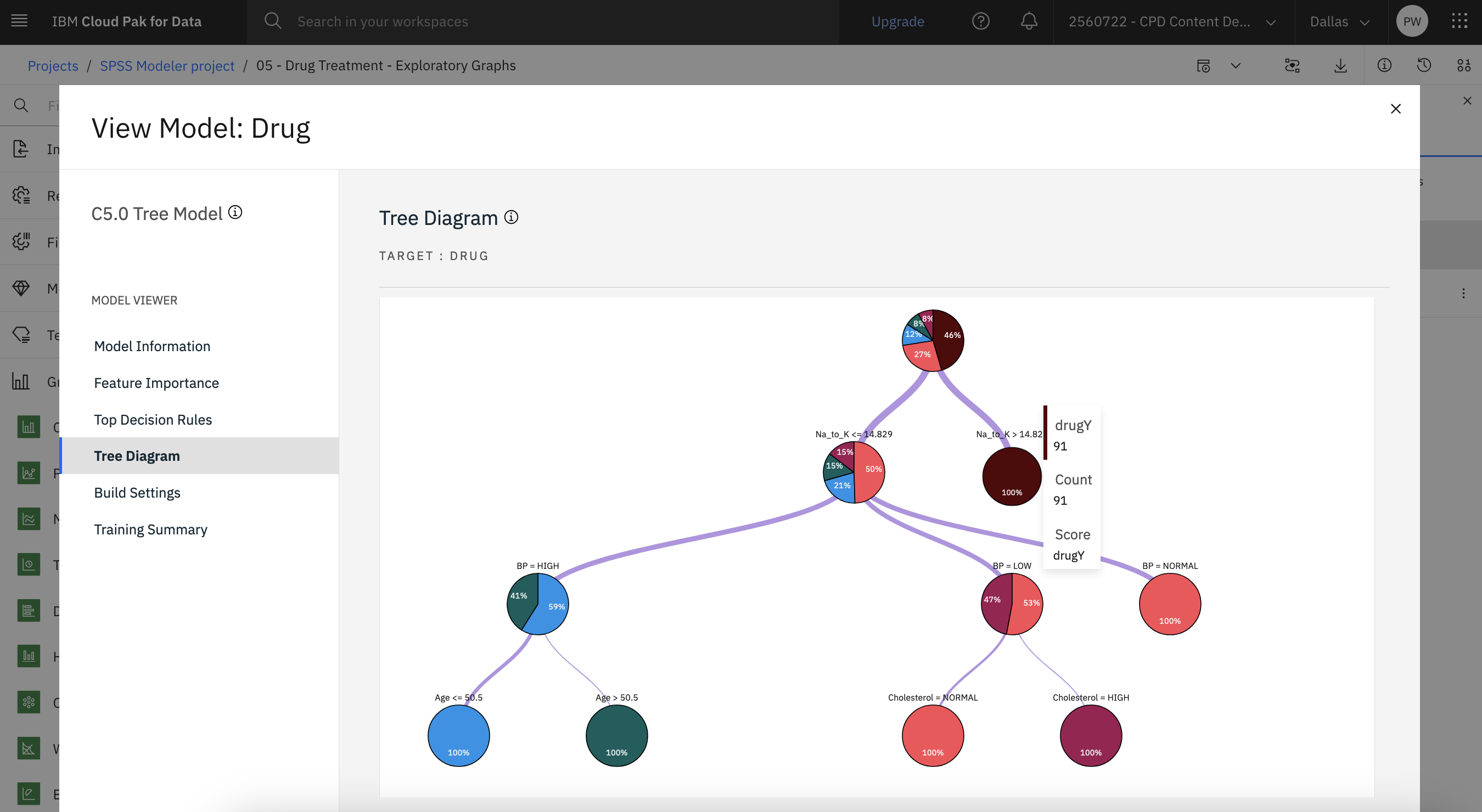
- In the Outputs and models pane, click the Drug model to view the results.
The Tree Diagram displays the set of rules that are generated by the C5.0 node in a tree format. Now, you can see the missing pieces of the puzzle. For people with an Na-to-K ratio less than
14.829You can hover over the nodes in the tree to see more details such as the number of cases for each blood pressure category and the confidence percentage of cases.
![]() Check your progress
Check your progress
The following image shows the tree diagram. You are now ready to create an Analysis node.
Task 10: Create an Analysis node
Follow these steps to assess the accuracy of the model by using an Analysis node:
- From the Outputs section in the palette, drag the Analysis node onto the canvas and connect it to the Drug (C5.0) model nugget.
- Hover over the Analysis node and click the Run icon
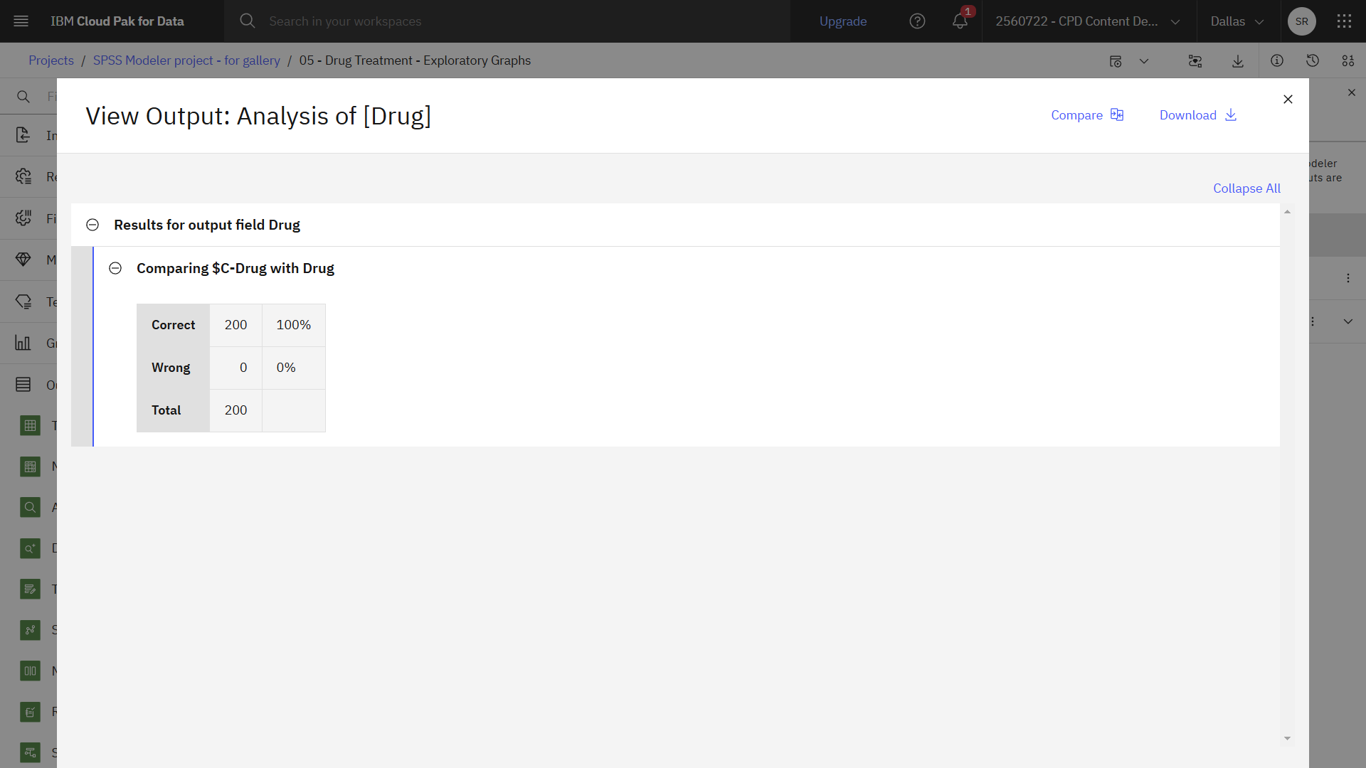
- In the Outputs and models pane, click the Analysis of [Drug] output to view the
results.
The Analysis node output shows that with this artificial dataset, the model correctly predicted the choice of drug for every record in the dataset. With a real dataset you are unlikely to see 100% accuracy, but you can use the Analysis node to help determine whether the model is acceptably accurate for your particular application.
![]() Check your progress
Check your progress
The following image shows Analysis output.
Summary
This example showed you how to create and explore graphs for drug treatment and use them to find out which drug might be appropriate for a future patient with the same illness.
Next steps
You are now ready to try other SPSS® Modeler tutorials.