This tutorial focuses on monitoring status information from a machine and the problem of recognizing and predicting fault states.
The data is created from a fictitious simulation and consists of several concatenated series that is measured over time. Each record is a snapshot report on the machine and includes the following fields:
Time. An integer.Power. An integer.Temperature. An integer.Pressure.0if normal,1for a momentary pressure warning.Uptime. Time since last serviced.Status. Normally0, changes to an error code if an error occurs (101,202, or303).Outcome. The error code that appears in this time series, or0if no error occurs. (These codes are available only with the benefit of hindsight.)
The following process is common to most data mining projects:
- Examine the data to determine which attributes might be relevant to the prediction or recognition of the states of interest.
- Retain those attributes (if already present), or derive and add them to the data, if necessary.
- Use the resultant data to train rules and neural nets.
- Test the trained systems by using independent test data.
Try the tutorial
In this tutorial, you will complete these tasks:
Sample modeler flow and data set
This tutorial uses the Condition Monitoring flow in the sample project. The data file used is cond1n.csv. The following image shows the sample modeler flow.

For each time series, there is a series of records from a period of normal operation followed by a period leading to the fault, as shown in the following image:

Task 1: Open the sample project
The sample project contains several data sets and sample modeler flows. If you don't already have the sample project, then refer to the Tutorials topic to create the sample project. Then follow these steps to open the sample project:
- In Cloud Pak for Data, from the Navigation menu
, choose Projects > View all Projects.
- Click SPSS Modeler Project.
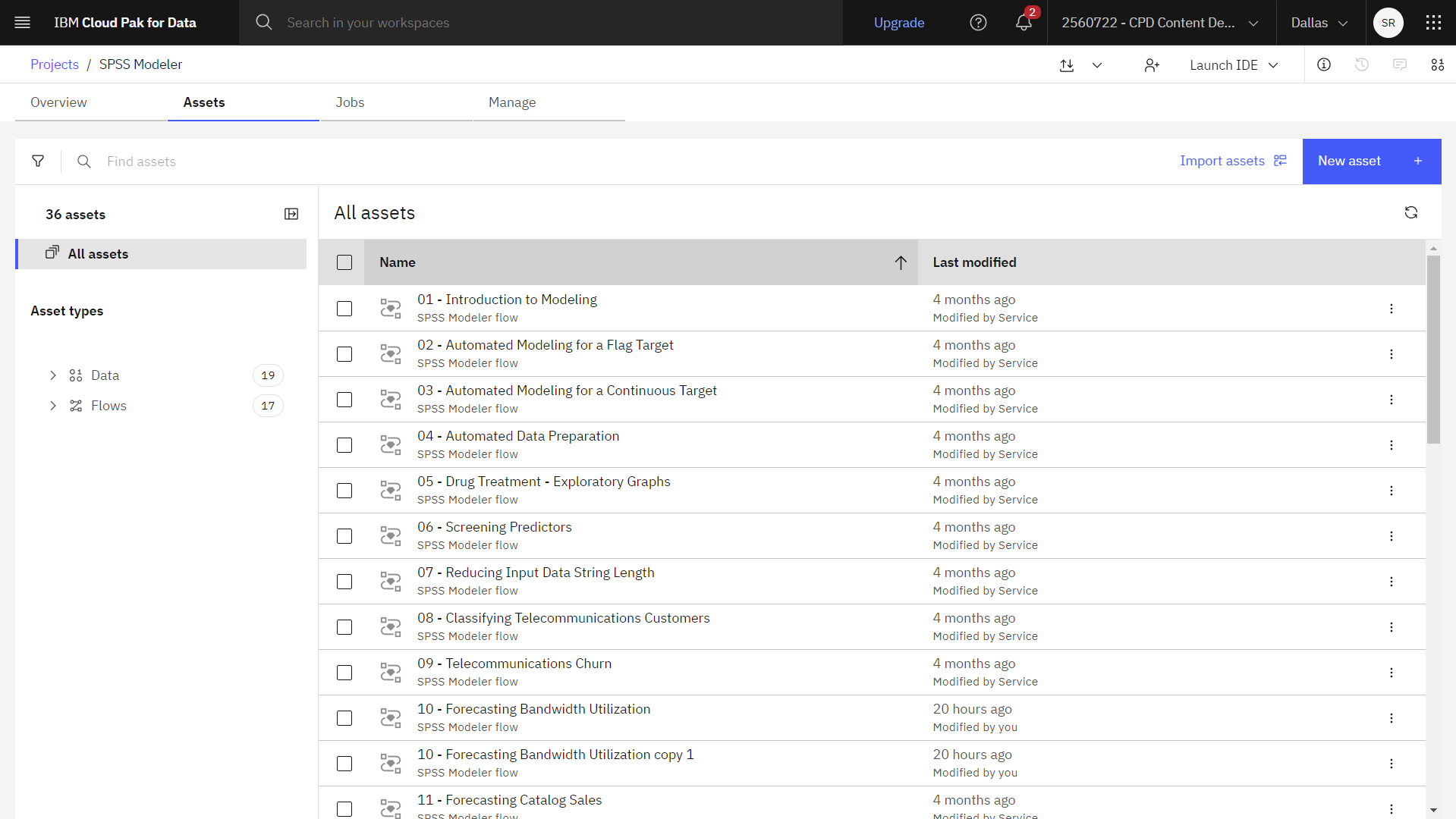
- Click the Assets tab to see the data sets and modeler flows.
Check your progress
The following image shows the project Assets tab. You are now ready to work with the sample modeler flow associated with this tutorial.

Task 2: Examine the Data Asset
Condition Monitoring modeler flow includes several nodes. Follow these steps to examine the Data Asset node:
- From the Assets tab, open the Condition Monitoring modeler flow, and wait for the canvas to load.
- Double-click the cond1n.csv node. This node is a Data Asset node that points to the cond1n.csv file in the project.
- Review the File format properties.
- From the Record Operations section in the palette, drag the Select node onto the
canvas. Hover over the node, click Edit Title, and rename it to
Select
(101)
. Connect it to the cond1n.csv data asset node. Double-click the Select node and enter a valueOutcome == 101for Condition. - Click Save.
- Next, from the Graph section in the palette, drag the Plot node onto the canvas. Hover over the node, click Edit Title button and rename it to Time v. Power v. Temperature (101). Then, connect it to the Select node.
- Double-click the Plot node and click the 3-D graph button to add a third axis to
your plot. From the list, select the fields to display on the 3-D graph. In this case:
Time,PowerandTemperature. - Hover over the Plot node and click the Run icon
 .
. - From the Outputs and models pane, click the output results with the name Time v. Power
v. Temperature (101) to view the results.
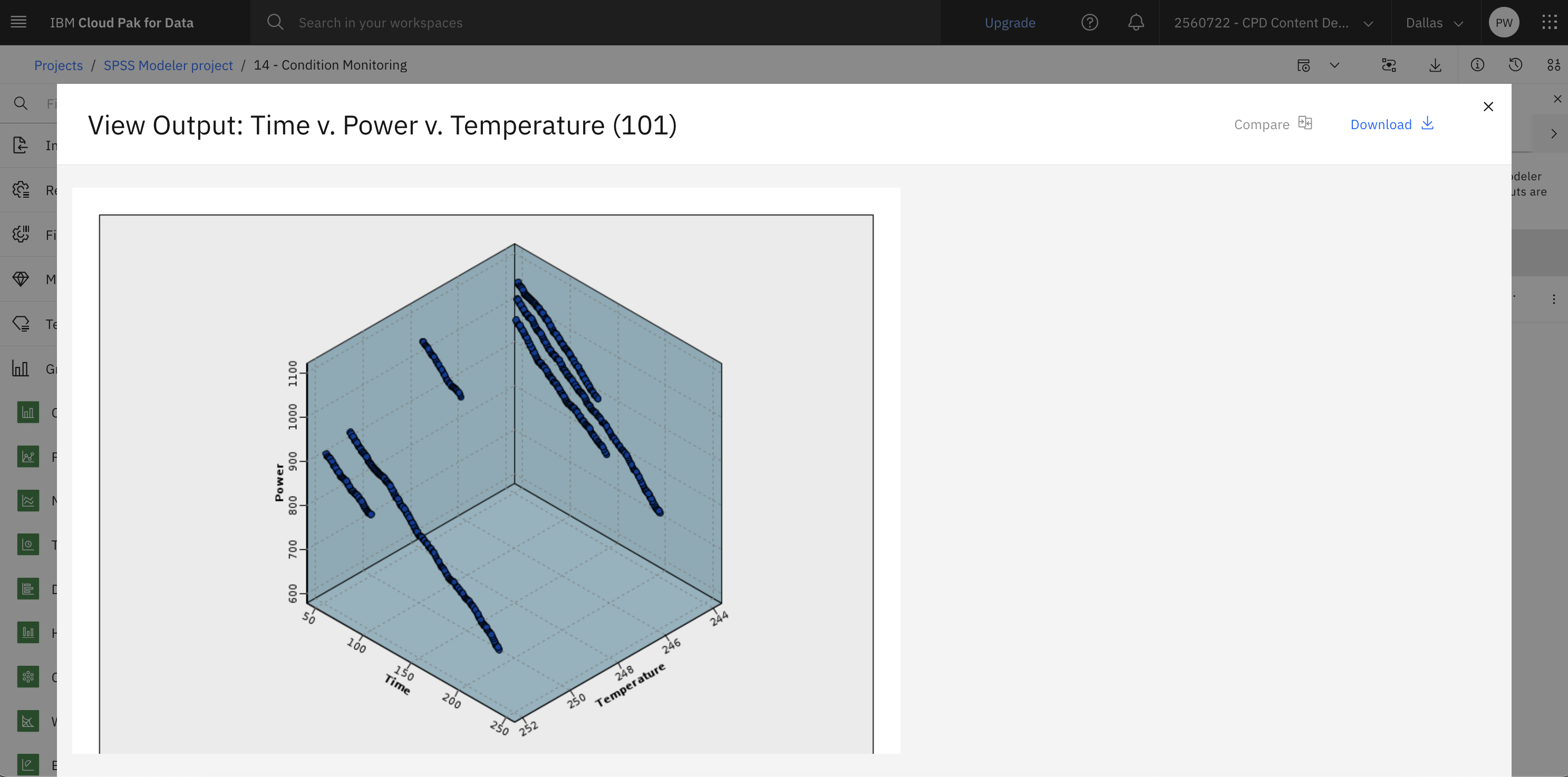
Figure 3. Time v. Power v. Temperature chart 
This graph shows 101 errors in rising temperature and fluctuating power over time. Experiment with selecting other error conditions and display other plots.
Based on these graphs, the presence and rate of change for both temperature and power, along with the presence and degree of fluctuation, are relevant to predicting and distinguishing faults. These attributes can be added to the data before applying the learning systems.
- Optional: Delete the Select and Plot nodes to avoid a potential error when the user runs the flow later on.
Check your progress
The following image shows the flow. You are now ready to prepare the data.

Task 3: Prepare the data
Based on the results of exploring the data, the following flow derives the relevant data and learns to predict faults.
This example uses the flow that is named Condition Monitoring, available in the example project installed with the product. The data files are cond1n.csv and cond2n.csv.
- Data Asset import node. Reads data file cond1n.csv.
- Pressure Warnings (Derive). Counts the number of momentary pressure warnings. Reset when time returns to 0.
- TempInc (Derive). Calculates the momentary rate of temperature change by
using
@DIFF1. - PowerInc (Derive). Calculates the momentary rate of power change by using
@DIFF1. - PowerFlux (Derive). A flag, true if power varied in opposite directions in the last record and this one; that is, for a power peak or trough.
- PowerState (Derive). A state that starts as
Stableand switches toFluctuatingwhen two successive power fluxes are detected. Switches back toStableonly when there is no power flux for five time intervals or whenTimeis reset. - PowerChange (Derive). Average of
PowerIncover the last five time intervals. - TempChange (Derive). Average of
TempIncover the last five time intervals. - Discard Initial (Select). Discards the first record of each time series
to avoid large (incorrect) jumps in
PowerandTemperatureat boundaries. - Discard fields (Filter). Cuts records down to
Uptime,Status,Outcome,Pressure Warnings,PowerState,PowerChange, andTempChange. - Type. Defines the role of
Outcomeas Target (the field to predict). In addition, defines the measurement level ofOutcomeas Nominal,Pressure Warningsas Continuous, andPowerStateas Flag.
Check your progress
The following image shows the Derive nodes. You are now ready to train the model.

Task 4: Train the model
Running the flow trains the C5.0 rule and neural network (net). The network might take some time to train, but training can be interrupted early to save a net that produces reasonable results. After the learning is complete, model nuggets are generated: one represents the neural net and one represents the rule.

These model nuggets enable you to test the system or export the results of the model. In this example, you test the results of the model. Follow these steps to train the model:
- Click Run all, and generate both the C5.0 and Neural network models.
- View each of the models. Double-click the Outcome (C5.0) model and click View model to check the results. Repeat this step for the Outcome (Neural Net) model.
Check your progress
The following image shows the model outcomes. You are now ready to test the model.

Task 5: Test the model
Follow these steps to test the model:
- Reposition the nuggets, so that the Type node connects to the neural net nugget, which connects to the C5.0 nugget.
- From the Outputs section in the palette, drag the Analysis node onto the canvas, and connect it to the C5.0 nugget.
- Double-click the Data Asset node.
- Click Change data asset.
- Select Data asset > cond2n.csv.
- Click Select.
- Click Save.
- Hover over the Analysis node and click the Run icon
 . Doing so yields figures reflecting the accuracy of the
trained network and rule.
 - From the Outputs and models pane, click the output results with the name Analysis to view the results.
- Review the results and compare the analysis for each model.
Figure 5. View Output: Analysis of [Outcome] ![View Output: Analysis of [Outcome]](/docs/api//content/wsd/tutorials/../images/condition-outputs-analysis.png?context=cpdaas&locale=en)
Check your progress
The following image shows the completed flow.

Summary
This example showed you how to monitor status information from a machine as it relates to the problems of recognizing and predicting fault states. You used a series of Derive nodes to prepare the data, and then built a C5.0 model.
Next steps
You are now ready to try other SPSS® Modeler tutorials.