This tutorial uses the Auto Classifier node to create automatically and compare a number of different models for either flag (such as whether a specific customer is likely to default on a loan or respond to a particular offer) or nominal (set) targets.
In this example, you search for a flag (yes or no) outcome. Within a relatively simple flow, the node generates and ranks a set of candidate models, chooses the ones that perform the best, and combines them into a single aggregated (Ensembled) model. This approach combines the ease of automation with the benefits of combining multiple models, which often yield more accurate predictions than can be gained from any one model.
This example is based on a fictional company that wants to achieve more profitable results by matching the appropriate offer to each customer. This approach stresses the benefits of automation. For a similar example that uses a continuous (numeric range) target, see the other SPSS® Modeler tutorials.
Try the tutorial
In this tutorial, you will complete these tasks:
Sample modeler flow and data set
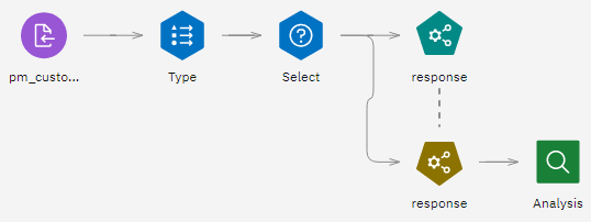
This tutorial uses the Automated Modeling for a Flag Target flow in the sample project. The data file used is pm_customer_train1.csv. The following image shows the sample modeler flow.
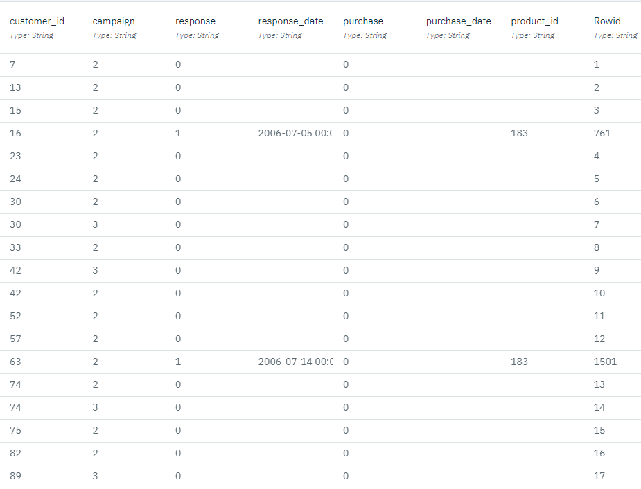
This example uses the data file pm_customer_train1.csv, which contains historical data
that tracks the offers made to specific customers in past campaigns, as indicated by the value of
the campaign field.
Task 1: Open the sample project
The sample project contains several data sets and sample modeler flows. If you don't already have the sample project, then refer to the Tutorials topic to create the sample project. Then follow these steps to open the sample project:
- In Cloud Pak for Data, from the Navigation menu
, choose Projects > View all Projects.
- Click SPSS Modeler Project.
- Click the Assets tab to see the data sets and modeler flows.
Check your progress
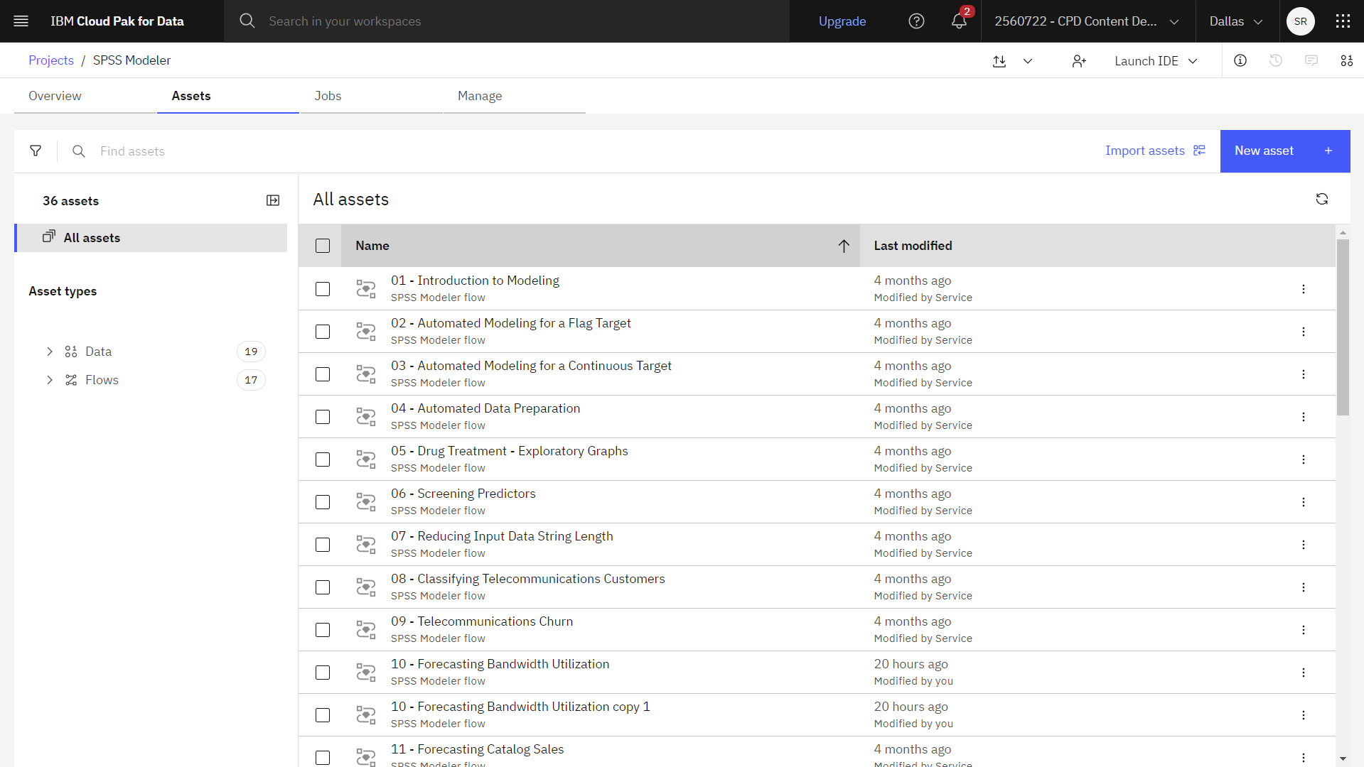
The following image shows the project Assets tab. You are now ready to work with the sample modeler flow associated with this tutorial.
Task 2: Examine the Data Asset node
Automated Modeling for a Flag Target includes several nodes. Follow these steps to examine the Data Asset node.
- From the Assets tab, open the Automated Modeling for a Flag Target modeler flow, and wait for the canvas to load.
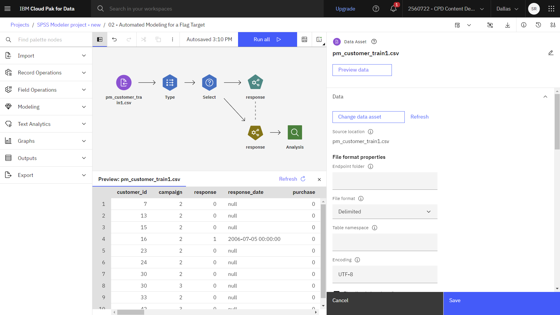
- Double-click the pm_customer_train1.csv node. This node is a Data Asset node that points to the pm_customer_train1.csv file in the project.
- Review the File format properties.
- Optional: Click Preview data to see the full data set.
The largest number of records fall under the Premium account campaign. The values of the
campaignfield are coded as integers in the data (for example2 = Premium account). Later, you define labels for these values that you can use to give more meaningful output.The file also includes a
responsefield that indicates whether the offer was accepted (0 = no, and1 = yes). Theresponsefield is the target field, or value, that you want to predict. Various fields containing demographic and financial information about each customer are also included. These fields are used to build or train a model that predicts response rates for individuals or groups based on characteristics such as income, age, or number of transactions per month.
Check your progress
The following image shows the Data Asset node. You are now ready to edit the Type node.
Task 3: Edit the Type node
Now that you explored the data asset, follow these steps to view and edit the properties of the Type node:
- Double-click the Type node. This node specifies field properties, such as measurement
level (the type of data that the field contains), and the role of each field as a target or input in
modeling. The measurement level is a category that indicates the type of data in the field. The
source data file uses three different measurement levels:
- A Continuous field (such as the
Agefield) contains continuous numeric values. - A Nominal field (such as the
Educationfield) has two or more distinct values; in this case.CollegeorHigh school. - An Ordinal field (such as the
Income levelfield) describes data with multiple distinct values that have an inherent order; in this case,Low,Medium, andHigh.
- A Continuous field (such as the
- Verify that the # response field is the target field (Role =
Target), and the measure for this field to Flag.
Figure 3. Set the measurement level and role 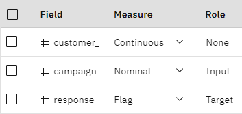
- Verify that the role to is set to None for the
following fields. These fields are ignored when you are building the model.
- customer_id
- campaign
- response_date
- purchase
- purchase_date
- product_id
- Rowid
- X_random
- Click Read Values in the Type node to make
sure that values are instantiated.
As you saw earlier, the source data includes information about four different campaigns, each targeted to a different type of customer account. These campaigns are coded as integers in the data, so to assist with remembering which account type each integer represents, define labels for each one.
Figure 4. Choose to specify values for a field 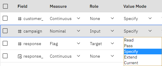
- In the # campaign row and the Value Mode column, select Specify from the list.
- Click the Edit icon
in the row for the # campaign field.
- Verify the labels as shown for each of the four values.
Figure 5. Define labels for the field values 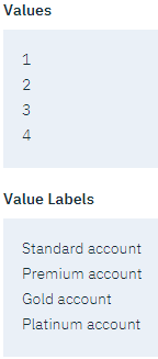
- Click OK. Now, the labels are displayed in output windows instead of the integers.
- Verify the labels as shown for each of the four values.
- Click Save.
- Optional: Click Preview data to see the data set with the Type properties applied.
Check your progress
The following image shows the Type node. You are now ready to select one campaign to analyze.

Task 4: Select one campaign to analyze
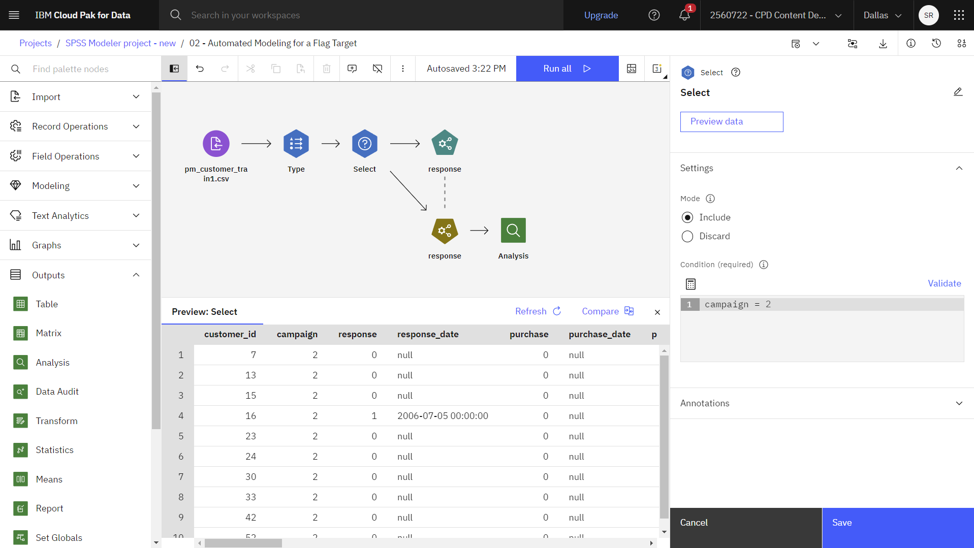
Although the data includes information about four different campaigns, you focus the analysis on one campaign at a time. Follow these steps to view the Select node to analyze just the Premium account campaign:
- Double-click the Select node to view its properties.
- Notice the Condition. Since the largest number of records fall under the Premium account
campaign (coded
campaign=2in the data), the Select node selects only these records. - Optional: Click Preview data to see the data set with the Select properties applied.
Check your progress
The following image shows the Select node. You are now ready to build the model.
Task 5: Build the model
Now that you have selected a single campaign to analyze, follow these steps to build the model that uses the Auto Classifier node:
- Double-click the Response (Auto Classifier) node to view its properties.
- Expand the Build Options section.
- In the Rank models by field, select Overall accuracy as the metric used to rank models.
- Set the Number of models to use to
3. This option means that the three best models are built when you run the node.Figure 6. Auto Classifier node, Build Options 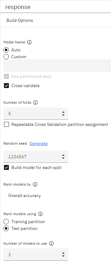
- Expand the Expert section to see the different modeling algorithms.
- Clear the Discriminant, SVM, and Random
Forest model types. These models take longer to train on this data, so eliminating them
speeds up the example.
Because you set the Number of models to use property to
3under Build Options, the node calculates the accuracy of the remaining algorithms and generate a single model nugget containing the three most accurate.Figure 7. Auto Classifier node, Expert options 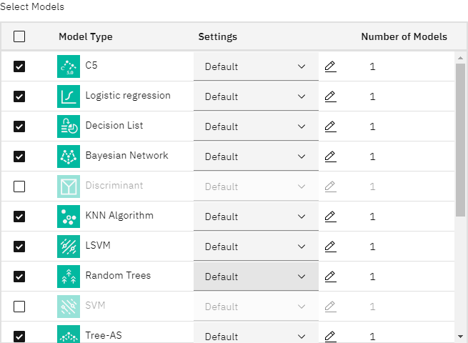
- Under the Ensemble options, select Confidence-weighted
voting for the ensemble method for both Set Targets and Flag Targets. This
setting determines how a single aggregated score is produced for each record.
With simple voting, if two out of three models predict yes, then yes wins by a vote of 2 to 1. In the case of confidence-weighted voting, the votes are weighted based on the confidence value for each prediction. Thus, if one model predicts no with a higher confidence than the two yes predictions combined, then no wins.
Figure 8. Auto Classifier node, Ensemble options 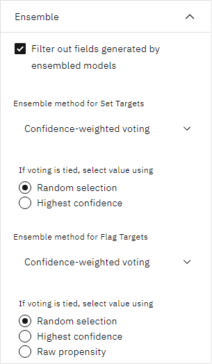
- Click Save.
- Hover over the Response (Auto Classifier) node, and click the Run icon
.
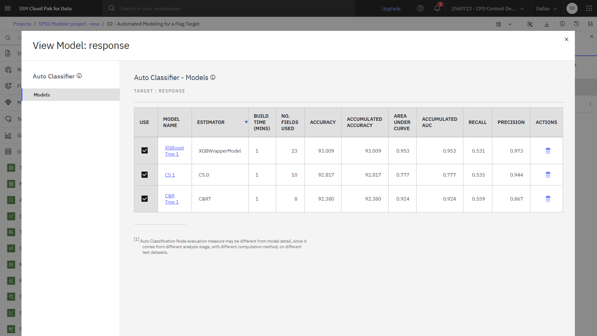
- In the Outputs and models pane, click the model with the name response to view the results. You see details about each of the models that are created during the run. (In a real situation, in which hundreds of models might be created on a large dataset, running the flow might take many hours.)
- Click a model name to explore any of the individual models results.
By default, models are sorted based on overall accuracy because you selected that measure in the Auto Classifier node properties. The XGBoost Tree model ranks best by this measure, but the C5.0 and C&RT models are nearly as accurate.
Based on these results, you decide to use all three of these most accurate models. By combining predictions from multiple models, limitations in individual models might be avoided, resulting in a higher overall accuracy.
- In the USE column, verify that all three models, and then close the model window.
Check your progress
The following image shows the model comparison table. You are now ready to run the model analysis.
Task 6: Run a model analysis
Now that you reviewed the generated models, follow these steps to run an analysis of the models:
- Hover over the Analysis node, and click the Run icon
.
- In the Outputs and models pane, click the Analysis output to view the results.
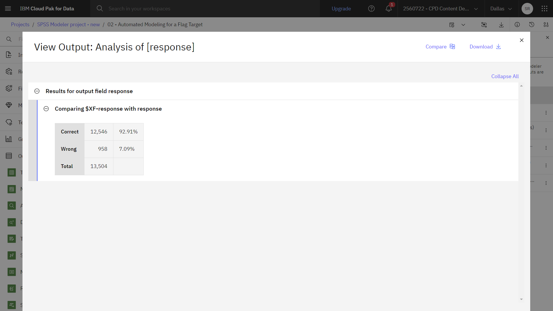
The aggregated score that is generated by the ensembled model is shown in a field named
$XF-response. When measured against the training data, the predicted value matches the actual response (as recorded in the originalresponsefield) with an overall accuracy of 92.77%. While not quite as accurate as the best of the three individual models in this case (92.82% for C5.0), the difference is too small to be meaningful. In general terms, an ensembled model will typically be more likely to perform well when applied to datasets other than the training data.
Check your progress
The following image shows the model comparison that uses the Analysis node.
Summary
With this example Automated Modeling for a Flag Target flow, you used the Auto Classifier node to compare several different models, used the three most accurate models, and added them to the flow within an ensembled Auto Classifier model nugget.
- Based on overall accuracy, the XGBoost Tree, C5.0, and C&R Tree models performed best on the training data.
- The ensembled model performed nearly as well as the best of the individual models and might perform better when applied to other datasets. If your goal is to automate the process as much as possible, this approach assists in obtaining a robust model under most circumstances without having to dig deeply into the specifics of any one model.
Next steps
You are now ready to try other SPSS Modeler tutorials.