- Run the flow. A generated model nugget is built and placed on the canvas, and results are added to the Outputs panel. You can view the model nugget, or save or deploy it in a number of ways.
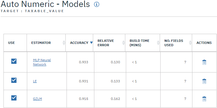
Hover over the model nugget, then click the overflow menu  and select View Model. You'll see
details about each of the models created during the run. (In a real situation, in which hundreds of
models are estimated on a large dataset, this could take many hours.)

If you want to explore any of the individual models further, you can click a model name in the ESTIMATOR column to drill down and explore the individual model results.

By default, models are sorted by accuracy (correlation) because correlation this was the measure you selected in the Auto Numeric node's properties. For purposes of ranking, the absolute value of the accuracy is used, with values closer to 1 indicating a stronger relationship.
You can sort on a different column by clicking the header for that column.
Based on these results, you decide to use all three of these most accurate models. By combining predictions from multiple models, limitations in individual models may be avoided, resulting in a higher overall accuracy.
In the USE column, make sure all three models are selected.
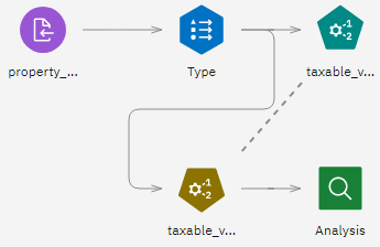
Attach an Analysis node (from the Outputs palette) after the model nugget. Hover over the Analysis node and click the Run icon ![]() to run the flow again.
to run the flow again.

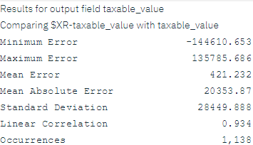
The averaged score generated by the ensembled model is added in a field named
$XR-taxable_value, with a correlation of 0.934, which is higher than those of the
three individual models. The ensemble scores also show a low mean absolute error and may perform
better than any of the individual models when applied to other datasets.
