This tutorial uses the Auto Numeric node to automatically create and compare different models for continuous (numeric range) outcomes, such as predicting the taxable value of a property. With a single node, you can estimate and compare a set of candidate models and generate a subset of models for further analysis. The node works in the same manner as the Auto Classifier node, but for continuous rather than flag or nominal targets.
The node combines the best of the candidate models into a single aggregated (Ensembled) model nugget. This approach combines the ease of automation with the benefits of combining multiple models, which often yield more accurate predictions than can be gained from any one model.
This example focuses on a fictional municipality responsible for adjusting and assessing real estate taxes. To accomplish this goal more accurately, you build a model that predicts property values based on building type, neighborhood, size, and other known factors.
Preview the tutorial
 Watch this video to preview the steps in this tutorial. There might
be slight differences in the user interface that is shown in the video. The video is intended to be
a companion to the written tutorial. This video provides a visual method to learn the concepts and
tasks in this documentation.
Try the tutorial
In this tutorial, you will complete these tasks:
Sample modeler flow and data set
This tutorial uses the Automated Modeling for a Continuous Target flow in the sample project. The data file used is property_values_train.csv. The following image shows the sample modeler flow.

The data file includes a field that is named taxable_value, which is the
target field, or value, that you want to predict. The other fields contain information
such as neighborhood, building type, and interior volume, and might be used as predictors.
| Field name | Label |
|---|---|
property_id |
Property ID |
neighborhood |
Area within the city |
building_type |
Type of building |
year_built |
Year built |
volume_interior |
Volume of interior |
volume_other |
Volume of garage and extra buildings |
lot_size |
Lot size |
taxable_value |
Taxable value |

Task 1: Open the sample project
The sample project contains several data sets and sample modeler flows. If you don't already have the sample project, then refer to the Tutorials topic to create the sample project. Then follow these steps to open the sample project:
- In Cloud Pak for Data, from the Navigation menu
, choose Projects > View all Projects.
- Click SPSS Modeler Project.
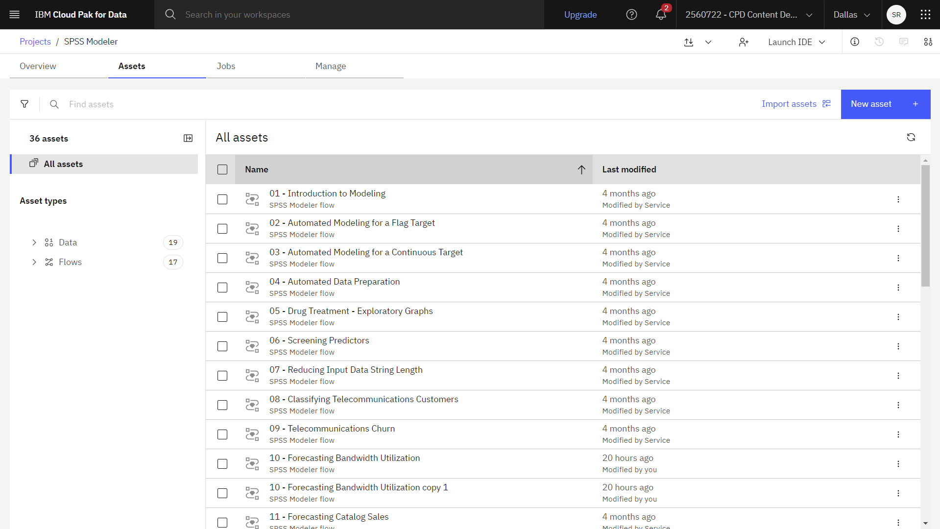
- Click the Assets tab to see the data sets and modeler flows.
Check your progress
The following image shows the project Assets tab. You are now ready to work with the sample modeler flow associated with this tutorial.

Task 2: Examine the Data Asset and Type nodes
Automated Modeling for a Continuous Target includes several nodes. Follow these steps to examine the Data Asset and Type nodes:
- From the Assets tab, open the Automated Modeling for a Continuous Target modeler flow, and wait for the canvas to load.
- Double-click the property_values_train.csv node. This node is a Data Asset node that points to the property_values_train.csv file in the project.
- Review the File format properties.
- Optional: Click Preview data to see the full data set.
- Double-click the Type node.
- For the taxable_value field, set the Role to Target. Other fields are used
as predictors.
Figure 3. Set the measurement level and role 
- Optional: Click Preview data to see the filtered data set.
Check your progress
The following image shows the Type node. You are now ready to configure the Modeling node.

Task 3: Configure the Modeling node
This example uses an Auto Numeric Modeling node which estimates and compares models to try out various approaches for a continuous numeric range. Follow these steps to configure the Modeling node:
- Double-click the taxable-value node to see its properties.
- Expand the Basics section, and set the following properties:
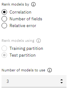
- For the Rank models by field, select Correlation.
- For the Number of models to use field, type
3. This means that the three best models will be built when you run the node.
Figure 4. Auto Numeric node Basics section 
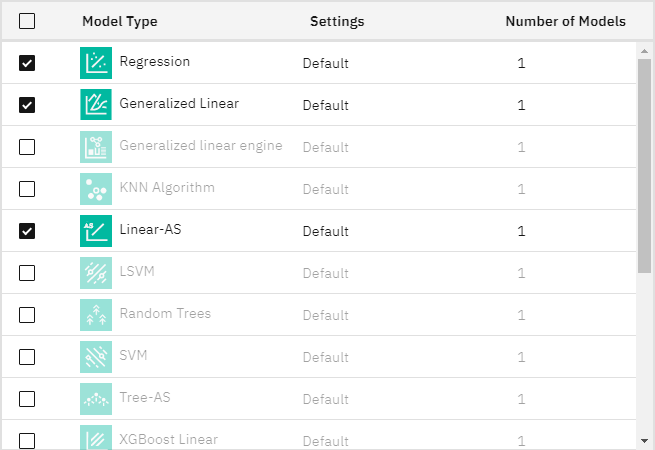
- Expand the Expert section. There are six algorithms that are selected which results in
the node estimating a single model for each algorithm, for a total of six models. (Alternatively,
you can modify these settings to compare multiple variants for each model type.) Because you set the
Number of models to use property to
3in the Basics section, the node calculates the accuracy of the six algorithms and build a single model nugget containing the three most accurate.Figure 5. Auto Numeric node Expert section 
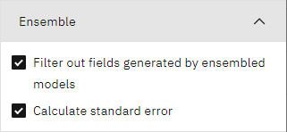
- Expand the Ensemble section to view the default settings. Since you use a continuous
target in this example, the ensemble score is generated by averaging the scores for the individual
models.
Figure 6. Auto Numeric node Ensemble section 
Check your progress
The following image shows the Modeling node. You are now ready to compare the models.

Task 4: Compare the models
Now that you specified the three models to build, follow these steps to generate and compare the models:
- Hover over the taxable_value node, and click the Run icon
.
- In the Outputs and models pane, click the results with the name taxable_value to
view the results.
You'll see details about each of the models that are created during the run. (In a real situation, in which hundreds of models are estimated on a large dataset, running the flow might take many hours.) The table contains a set of models that are generated by the Modeling node.
- To explore any of the individual models further, click a model name in the Estimator
column to see the individual model results.
- View the Model Information page. This table contains information on the type of model that is fitted, identifies the target field, the number of input features, activation functions, and the size of the resulting network.
- View any other pages for the model.
- Close the model details.
By default, models are sorted by accuracy (correlation) because you selected correlation as the measure in the Auto Numeric node's properties. For purposes of ranking, the absolute value of the accuracy is used, with values closer to 1 indicating a stronger relationship.
You can sort on a different column by clicking the header for that column.
Based on these results, you decide to use all three of these most accurate models. By combining predictions from multiple models, limitations in individual models might be avoided, resulting in a higher overall accuracy.
- Verify that all three models are selected in the Use column.
- Close the View Model: taxable_value window.
Check your progress
The following image shows the model comparison table. You are now ready to run the model analysis.

Task 5: Run the Analysis node
Now that you viewed a comparison of the three models, you can follow these steps to run an analysis of the models:
- Hover over the Analysis node, and click the Run icon
.
- In the Outputs and models pane, click the output results with the name Analysis to
view the results.
The averaged score that is generated by the ensembled model is added in a field that is named
$XR-taxable_value, with a correlation of 0.934, which is higher than those scores of the three individual models. The ensemble scores also show a low mean absolute error and might perform better than any of the individual models when applied to other datasets.
Check your progress
The following image shows the model comparison from the Analysis node.

Summary
With this example Automated Modeling for a Flag Target flow, you used the Auto Numeric node to compare several different models, selected the three most accurate models, and added them to the flow within an ensembled Auto Numeric model nugget.
The ensembled model showed performance that was better than two of the individual models and might perform better when applied to other datasets. If your goal is to automate the process as much as possible, this approach assists with obtaining a robust model under most circumstances without having to dig deeply into the specifics of any one model.
Next steps
You are now ready to try other SPSS® Modeler tutorials.