About cookies on this site Our websites require some cookies to function properly (required). In addition, other cookies may be used with your consent to analyze site usage, improve the user experience and for advertising. For more information, please review your options. By visiting our website, you agree to our processing of information as described in IBM’sprivacy statement. To provide a smooth navigation, your cookie preferences will be shared across the IBM web domains listed here.
Last updated: Feb 12, 2025
As a result of IBM research, and inspired by natural selection in biology, continuous machine learning is available for the Auto Classifier node and the Auto Numeric node.
An inconvenience with modeling is models getting outdated due to changes to your data over time. This is commonly referred to as model drift or concept drift. To help overcome model drift effectively, SPSS Modeler provides continuous automated machine learning.
What is model drift? When you build a model based on historical data, it can become stagnant. In many cases, new data is always coming in—new variations, new patterns, new trends, etc.—that the old historical data doesn't capture. To solve this problem, IBM was inspired by the famous phenomenon in biology called the natural selection of species. Think of models as species and think of data as nature. Just as nature selects species, we should let data select the model. There's one big difference between models and species: species can evolve, but models are static after they're built.
There are two preconditions for species to evolve; the first is gene mutation, and the second is population. Now, from a modeling perspective, to satisfy the first precondition (gene mutation), we should introduce new data changes into the existing model. To satisfy the second precondition (population), we should use a number of models rather than just one. What can represent a number of models? An Ensemble Model Set (EMS)!
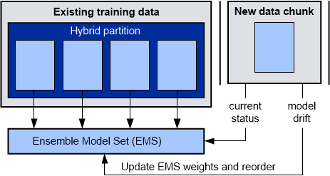
The following figure illustrates how an EMS can evolve. The upper left portion of the figure represents historical data with hybrid partitions. The hybrid partitions ensure a rich initial EMS. The upper right portion of the figure represents a new chunk of data that becomes available, with vertical bars on each side. The left vertical bar represents current status, and the right vertical bar represents the status when there's a risk of model drift. In each new round of continuous machine learning, two steps are performed to evolve your model and avoid model drift.
First, you construct an ensemble model set (EMS) using existing training data. After that, when a new chunk of data becomes available, new models are built against that new data and added to the EMS as component models. The weights of existing component models in the EMS are reevaluated using the new data. As a result of this reevaluation, component models having higher weights are selected for the current prediction, and component models having lower weights may be deleted from the EMS. This process refreshes the EMS for both model weights and model instances, thus evolving in a flexible and efficient way to address the inevitable changes to your data over time.
The ensemble model set (EMS) is a generated auto model nugget, and there's a refresh link between the auto modeling node and the generated auto model nugget that defines the refresh relationship between them. When you enable continuous auto machine learning, new data assets are continuously fed to auto modeling nodes to generate new component models. The model nugget is updated instead of replaced.
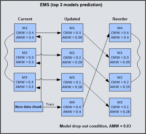
The following figure provides an example of the internal structure of an EMS in a continuous machine learning scenario. Only the top three component models are selected for the current prediction. For each component model (labeled as M1, M2, and M3), two kinds of weights are maintained. Current Model Weight (CMW) describes how a component model performs with a new chunk of data, and Accumulated Model Weight (AMW) describes the comprehensive performance of a component model against recent chunks of data. AMW is calculated iteratively via CMW and previous values of itself, and there's a hyper parameter beta to balance between them. The formula to calculate AMW is called exponential moving average.
When a new chunk of data becomes available, first SPSS Modeler uses it to build a few new component models. In this example figure, model four (M4) is built with CMW and AMW calculated during the initial model building process. Then SPSS Modeler uses the new chunk of data to reevaluate measures of existing component models (M1, M2, and M3) and update their CMW and AMW based on the reevaluation results. Finally, SPSS Modeler might reorder the component models based on CMW or AMW and select the top three component models accordingly.
In this figure, CMW is described using normalized value (sum = 1) and AMW is calculated based on CMW. In SPSS Modeler, the absolute value (equal to evaluation-weighted measure selected - for example, accuracy) is chosen to represent CMW and AMW for simplicity.
Note that there are two types of weights defined for each EMS component model, both of which
could be used for selecting top N models and component model drop out:
- Current Model Weight (CMW) is computed via evaluation against the new data chunk (for example, evaluation accuracy on the new data chunk).
- Accumulated Model Weight (AMW) is computed via combining both CMW and existing AMW
(for example, exponentially weighted moving average (EWMA).
Exponential moving average formula for calculating AMW:

In SPSS Modeler, after running an Auto Classifier node to generate a model nugget, the following model options are available for continuous machine learning:
- Enable continuous auto machine learning during model refresh. Select this option to enable continuous machine learning. Keep in mind that consistent metadata (data model) must be used to train the continuous auto model. If you select this option, other options are enabled.
- Enable automatic model weights reevaluation. This option controls whether
evaluation measures (accuracy, for example) are computed and updated during model refresh. If you
select this option, an automatic evaluation process will run after the EMS (during model refresh).
This is because it's usually necessary to reevaluate existing component models using new data to
reflect the current state of your data. Then the weights of the EMS component models are assigned
according to reevaluation results, and the weights are used to decide the proportion a component
model contributes to the final ensemble prediction. This option is selected by default.
Figure 3. Model settings 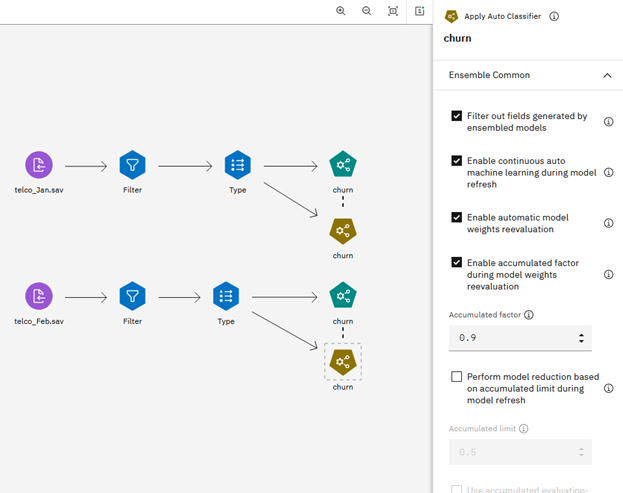
Figure 4. Flag target 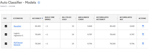 Following are the supported CMW and AMW for the Auto Classifier node:
Table 1. Supported CMW and AMW Target type CMW AMW flag target Overall Accuracy
Area Under CurveAccumulated Accuracy
Accumulated AUCset target Overall Accuracy Accumulated Accuracy The following three options are related to AMW, which is used to evaluate how a component model performs during recent data chunk periods:
- Enable accumulated factor during model weights reevaluation. If you select this option, AMW computation will be enabled during model weights reevaluation. AMW represents the comprehensive performance of an EMS component model during recent data chunk periods, related to the accumulated factor β defined in the AMW formula listed previously, which you can adjust in the node properties. When this option isn't selected, only CMW will be computed. This option is selected by default.
- Perform model reduction based on accumulated limit during model refresh.
Select this option if you want component models with an AMW value below the specified limit to be
removed from the auto model EMS during model refresh. This can be helpful in discarding component
models that are useless to prevent the auto model EMS from becoming too heavy.The accumulated limit value evaluation is related to the weighted measure used when Evaluation-weighted voting is selected as the ensemble method. See the following.
Figure 5. Set and flag targets 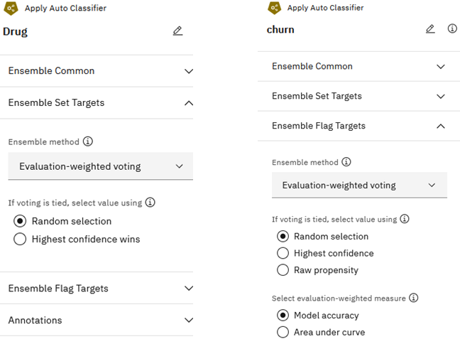
Note that if you select Model Accuracy for the evaluation-weighted measure, models with an accumulated accuracy below the specified limit will be deleted. And if you select Area under curve for the evaluation-weighted measure, models with an accumulated AUC below the specified limit will be deleted.
By default, Model Accuracy is used for the evaluation-weighted measure for the Auto Classifier node, and there's an optional AUC ROC measure in the case of flag targets.
- Use accumulated evaluation-weighted voting. Select this option if you
want AMW to be used for the current scoring/prediction. Otherwise, CMW will be used by default. This
option is enabled when Evaluation-weighted voting is selected for the
ensemble method.
Note that for flag targets, by selecting this option, if you select Model Accuracy for the evaluation-weighted measure, then Accumulated Accuracy will be used as the AMW to perform the current scoring. Or if you select Area under curve for the evaluation-weighted measure, then Accumulated AUC will be used as the AMW to perform the current scoring. If you don't select this option and you select Model Accuracy for the evaluation-weighted measure, then Overall Accuracy will be used as the CMW to perform the current scoring. If you select Area under curve, Area under curve will be used as the CMW to perform the current scoring.
For set targets, if you select this Use accumulated evaluation-weighted voting option, then Accumulated Accuracy will be used as the AMW to perform the current scoring. Otherwise, Overall Accuracy will be used as the CMW to perform the current scoring.
With continuous auto machine learning, the auto model nugget is evolving all the time by rebuilding the auto model, which ensures that you get the most updated version reflecting the current state of your data. SPSS Modeler provides the flexibility for different top N component models in the EMS to be selected according to their current weights, which keeps pace with varying data during different periods.
Note: The Auto Numeric node is a much simpler case, providing a subset of the options in the Auto
Classifier node.
Example
In this example, continuous machine learning is used in the telecommunications industry to predict behavior and retain customers.
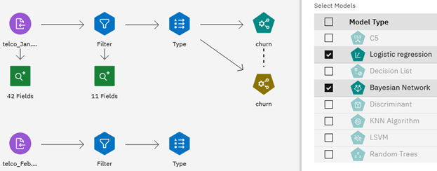
In the following flow, the data asset includes information about customers who left within the
last month (ChurnJanFeb
Now let's have a look at what's inside the auto model nugget. We can see it contains three component models for the three algorithms we selected. For each component model, there are several evaluation measures generated (such as accuracy and area under curve). These evaluation measures describe how a component model performs against training data (the January data set). You can select which component models to use in the current ensemble prediction.
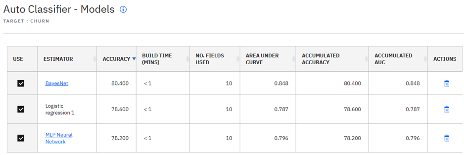
You may see accumulated evaluation measures, also. These accumulated measures are for continuous machine learning, as they describe how a component model performs with recent data changes, so that you're aware of the model's comprehensive performance over a period of time. As this is our initial auto model, we see that the initial values for the accumulated measures are the same as related current measures. By default, evaluation measures are calculated against training data, so there could be some degree of overfitting. To avoid this, the Auto Classifier node provides a build option that calculates more stable evaluation measures via cross validation.
Next, let's look at how the final ensemble prediction is generated. If we open an auto model's properties, under Ensemble Flag Targets, the training target churn field is a yes/no flag target. Under Ensemble Set Targets (for set target fields that contain more than two values), there's an Ensemble method drop-down. Several options are available in the drop-down (for example, Majority voting means each component model holds one ticket to vote, and Confidence-weighted voting means the confidence field of each component model's prediction is used as the voting weight—with higher confidence having more influence on the final ensemble prediction). Similarly, to enable better support for continuous machine learning, Evaluation-weighted voting is available so that the component model's evaluation measure (for example, model accuracy or area under curve) will be used as the voting weight. In the case of a flag target, there's also an option to select a specific evaluation measure as the voting weight when Evalution-weighted voting is used. In the case of a set target, only Accuracy is currently supported.
Under the Ensemble Common settings is where you turn on continuous machine learning. Then we can use the February data to see what's happening. We might select two different algorithms to distinguish between the existing component model algorithms. Then after rebuilding the flow and viewing the auto model's content, we see that two new component models are added (C5 and C&RT). We also notice that the evaluation measures for the existing component models have been recalculated. Both CMW measures and AMW measures are different than before. We can now compare them to the corresponding measures in the original auto model.
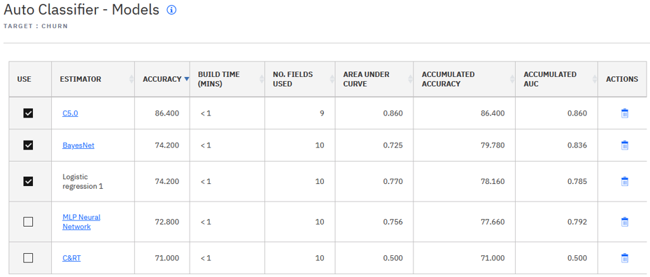
Now what? With the enhanced auto model, we can select a prioritized evaluation measure and get top-N component models ordered by that measure. Then we can use the top-N component models to participate in the final ensemble prediction for incoming predictive analytics requests. And if Evaluation-weighted voting is selected for the Ensemble method, we can use accumulated measures as voting weights by simply selecting the option Use accumulated evaluation-weighted voting under the Ensemble Common settings. If deselected, CMW measures will be used by default in evaluation-weighted voting.
With continuous machine learning, the auto model is evolving all the time as it is continuously rebuilding against new chunks of data, ensuring that your model is the most up-to-date version that reflects the current status of the data. This allows for the flexibility to select different top-N component models in the EMS according to their current or accumulated evaluation measures, to keep pace with varying data during different periods.
Periodically, you may choose to deploy the most up-to-date Auto model into Watson Machine Learning periodically for convenience.
Was the topic helpful?
0/1000